Bootcamp

Imagine we have an autonomous car that would like to perform speedy highway driving. There are several approaches to program such an autonomous vehicle. The first would be to hand-craft a rule-based system consisting of what to do in different scenarios. An example rule could be “if the autonomous car would like to move forward and there is a car in front and to the left, switch to the right lane”. A programmer could write down hundreds of rules consisting of every possible scenario. However, this process is expensive and leaves much to be desired. The second approach would be to utilize a driving simulator and design a reward function that defines the proper autonomous driving behavior. Then, one could use reinforcement learning to learn an optimal driving policy. However, defining such a reward function is difficult. Furthermore, if the driving simulator has differences with the real world, the behavior of the autonomous car may degrade when deployed. Lastly, one can utilize learning from demonstration (LfD), where user demonstrations are used directly to learn autonomous driving behavior. LfD has many benefits, including that it can learn human-like behavior and does not require a simulator. It is also much easier for a human to give an example of driving on the highway than defining all the rules used during driving. However, what happens when two drivers present demonstrations with conflicting behaviors (e.g., one prefers to pass on the left versus the other prefers to pass on the right)?

In this post, we are going to discuss how robots can learn from heterogeneous human demonstrators, demonstrators that will perform the same task in different ways.

This blog post will address the following questions in 3 parts:

1. What challenges arise from heterogeneity in demonstrations?
2. How can we automatically infer preferences within demonstrations?
3. How can we utilize person-specific embeddings in policy learning?

1. Challenges from heterogeneity of demonstrations

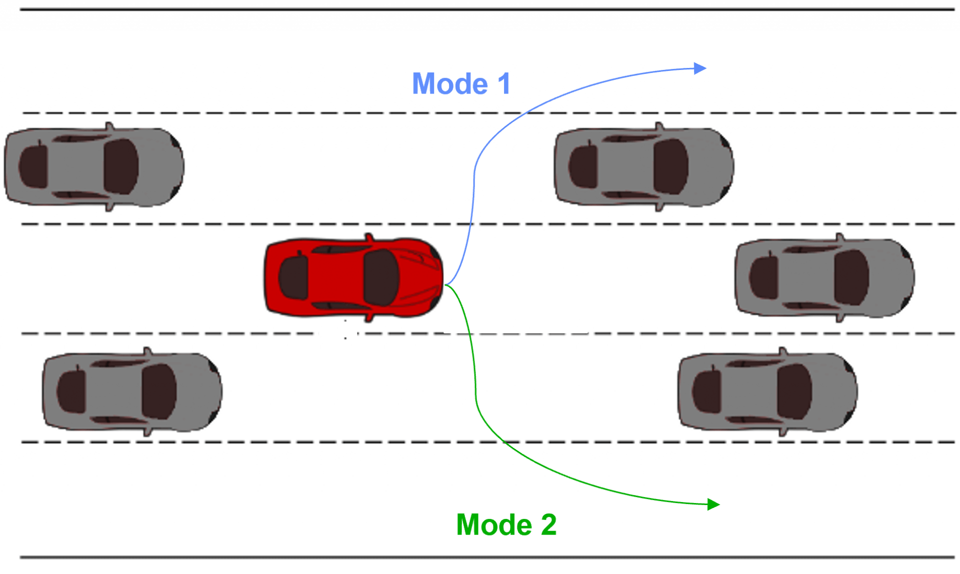
We can imagine multiple real-life scenarios, ranging from driving to the setting of a dinner table, in which there are heterogeneous approaches that can be utilized to reach the same goal. Continuing the autonomous driving example from the introduction, Figure 1 displays the heterogeneity that can occur within driving demonstrations. Within the example displayed, some subset of the demonstrators preferred to pass on the left while others preferred to pass on the right. LfD approaches that assume homogeneous demonstration will either fit to the mean (drive straight into the car in front) or fit a single-mode (only pass on one side), both producing suboptimal/limited driving behavior. It is important to model the heterogeneity within the Learning from Demonstration framework. We will accomplish this via variational inference for person-specific embeddings.

The decision-making we employ to select our approach can be explicitly defined as a policy; a function that maps states $S$ to actions $A$ (Equation 1).

\begin{align}
\hat{\pi}: S \rightarrow A
\end{align}

Depending on an implicit demonstrator preference, the demonstrator may find it advantageous to choose one policy over the other. For example, a demonstrator setting the table may be left-handed and prefer to set a drinking glass on the left-hand side. Without explicitly labeling demonstrations by preference, the context within this selection process is lost to a robot attempting to learn the task, making it very difficult to learn a policy representation across all demonstrators. Without access to latent information about demonstrators, current LfD approaches sacrifice optimal behavior for consistency, weaken the robustness of the robot to different scenarios, and reduce the number of examples the robot can use to learn from.

As we consider scenarios where the number of demonstrations is numerous, it becomes advantageous to be able to autonomously infer distinct modalities without requiring someone at hand to label each demonstration. In addition, we would also like to learn a policy representing user demonstrations within our dataset. How can one accomplish both objectives, inferring latent information about demonstrated trajectories and learning a policy conditioned upon contextual and latent information, simultaneously?

2. Inferring trajectory modalities

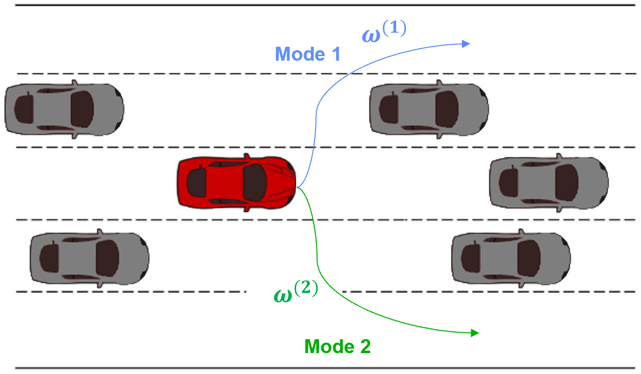
We seek to autonomously infer distinct strategies or modes $\omega$ from the real-world demonstrations we are able to acquire. Following our autonomous driving example, Figure 2 displays the end result we seek to achieve: mode 1 demonstrations are assigned a specific latent code and mode 2 demonstrations are assigned a different latent code. Visually, in Figure 2 it is clear that there are only two types of demonstrations. We would like our approach to discover first, that there are different modes within the demonstration data-set and second, how many modes are present.

To do so, we would like to maximize the mutual information $I$ between our embedding mode $\omega$ and the actions taken by our policy $\pi_\theta(a|\omega,s)$, where our policy is conditioned on the state and latent code. We display a representation of the mutual information in Equation 2, where H is the entropy function.

\begin{gather}
I(\omega;\pi(a|\omega,s)) = H(\omega) – H(\omega|\pi(a|\omega,s))
\end{gather}

Maximizing mutual information encourages $\omega$ to correlate with semantic features within the data distribution (i.e., mode discovery), which is exactly what we want! However, maximizing the mutual information between the trajectories and latent code is intractable as it requires access to the true posterior, $P(\omega|s,a)$, representing the distribution of modalities given trajectories. Instead, we can utilize a lower bound of the mutual information and maximize the lower-bound via gradient descent, thereby maximizing the mutual information and incentivizing the policy to utilize $\omega$ as much as possible.

Recall that the KL divergence is a measure of similarity between two probability distributions. We can express the KL divergence between $p$ and $q$ with Equation 3.

\begin{align}
D_{KL} \left( p (\omega | s, a) \ || \ q(\omega | s, a) \right) = \mathop{\mathbb{E}}_{\omega \sim p(\omega | s, a)} log \frac{p(\omega | s, a)}{ q(\omega|s,a)}
\end{align}

We display the derivation of the mutual information lower bound in Equation 4. Below, we provide a step-by-step walkthrough of the derivation.
\begin{align}
\begin{split}
I(\omega;\pi(a|\omega,s)) &= H(\omega) – H(\omega|\pi(a|\omega,s))) \\
&= H(\omega)-\mathop{\mathbb{E}}_{a \sim \pi(\cdot| \omega, s)}\big[\mathop{\mathbb{E}}_{\omega \sim p(\omega| s,a)} [- \log p(\omega|s,a)\big]] \\
&= H(\omega)+\mathop{\mathbb{E}}_{a \sim \pi(\cdot| \omega, s)}\big[\mathop{\mathbb{E}}_{\omega \sim p(\omega| s,a)} [\log p(\omega|s,a)\big]] \\
&= H(\omega)+D_{KL}(p(\omega|s,a)||q(\omega|s,a)) + \mathop{\mathbb{E}}_{a \sim \pi(\cdot| \omega, s)}\big[\mathop{\mathbb{E}}_{\omega \sim p(\omega| s,a)} [\log q(\omega|s,a)\big]] \\
&\geq H(\omega) + \mathop{\mathbb{E}}_{a \sim \pi(\cdot| \omega, s)}\big[\mathop{\mathbb{E}}_{\omega \sim p(\omega| s,a)} [\log q(\omega|s,a)\big]] \\
\end{split}
\end{align}

In line 1 of the derivation, we have Equation 2. To transition into line 2 of the derivation in Equation 4, we simplify the second entropy term. Line 3 of the derivation brings the negative sign outside of the expectation. Line 4 utilizes the identity $\mathop{\mathbb{E}}_{x \sim p_{X}(\cdot)}(p(x)) = D_{KL}(P||Q) + \mathop{\mathbb{E}}_{x \sim p_{X}(\cdot)}(q(x))$ in transitioning from line 3. Here, q is an approximate posterior for the true distribution of embeddings given trajectories. In transitioning to line 5, since the KL divergence between two distributions is always positive, we replace the equal sign with a greater than or equal to and remove the divergence term. We note that during optimization, we assume that the distribution of embeddings is a static, uniform distribution, and thus, the entropy across latent codes, $H(\omega)$ is constant and can be removed. Line 5 displays the final result, the lower bound of the mutual information.

Notice that we have now described a substitute objective function that is expressly in terms the latent mode variable $\omega$ and our approximate posterior $q$. Maximizing this objective should make different latent embeddings correspond with different policy behaviors. However, one problem remains: our computation of $q$ is based on the sampling over the expectation of the true posterior p($\omega$|s,a), which is still unknown. Therefore, we seek to gradually tease out the true distribution while training through sampling. We denote $\omega$, the discovered latent codes, as person-specific embeddings as each embedding displays latent features for a specific demonstrator.

3. Simultaneously learning a policy while inferring person-specific embeddings

Our goal is to learn demonstrator policies that are conditioned on person-specific embeddings, $\omega$. Thus, even if heterogeneity is present with the demonstrations, the latent encodings will be able to represent the unique behaviors among demonstrators. The resultant policy is able to adapt to a person’s unique characteristics while simultaneously leveraging any homogeneity that exists within the data (e.g., uniform adherence to hard constraints).

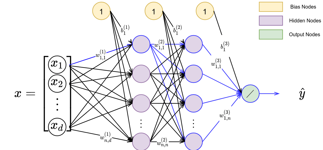
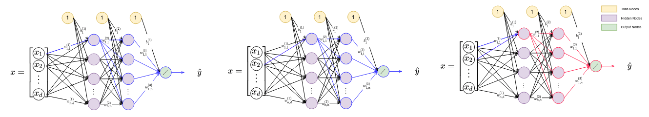
Accordingly, we will want to maximize our ability to imitate demonstrators via a behavior cloning loss and the mutual information between person-specific embeddings and trajectories via a variational information maximization (VIM) loss. We display a general overview of the architecture used during learning from heterogeneous demonstration in Figure 3.

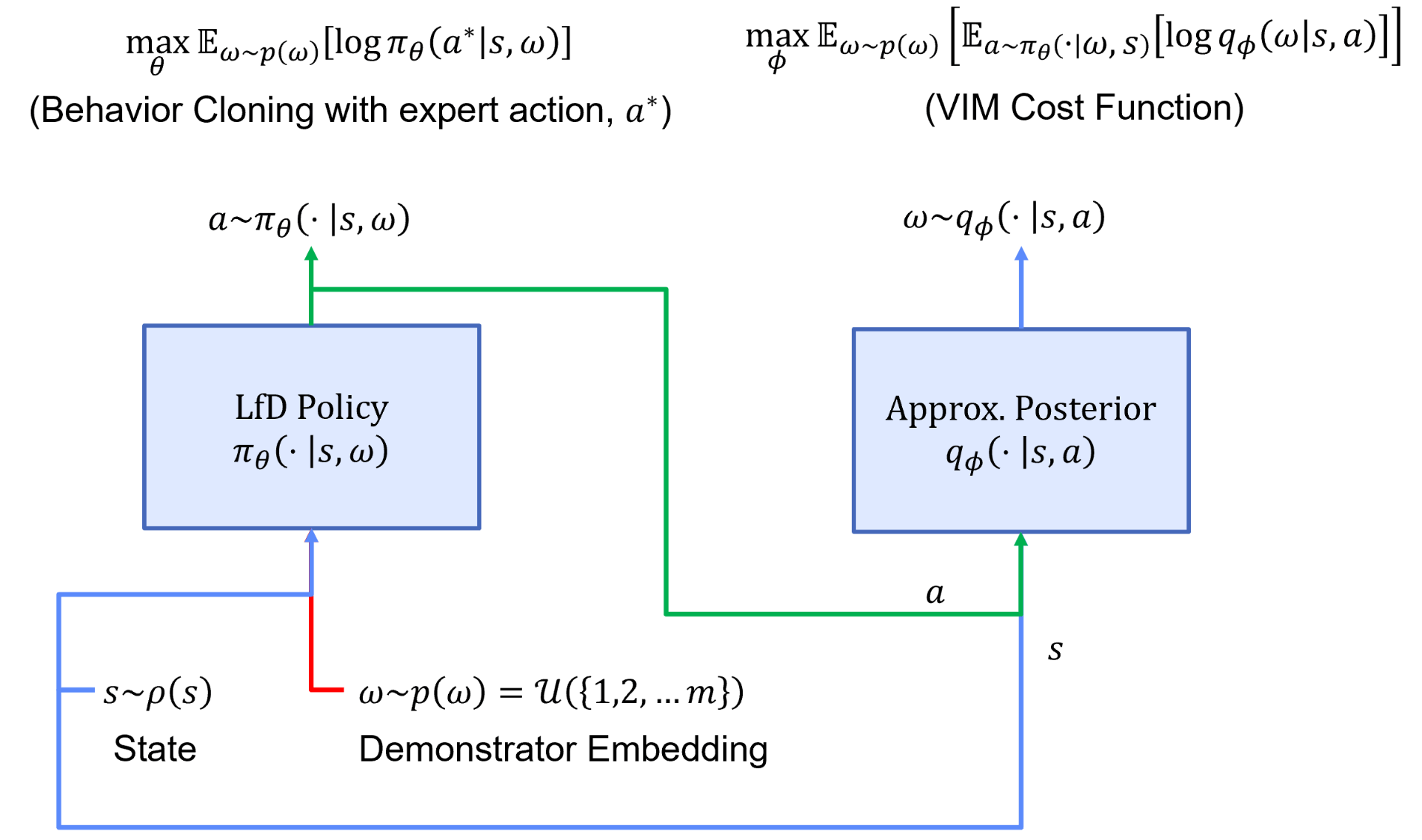
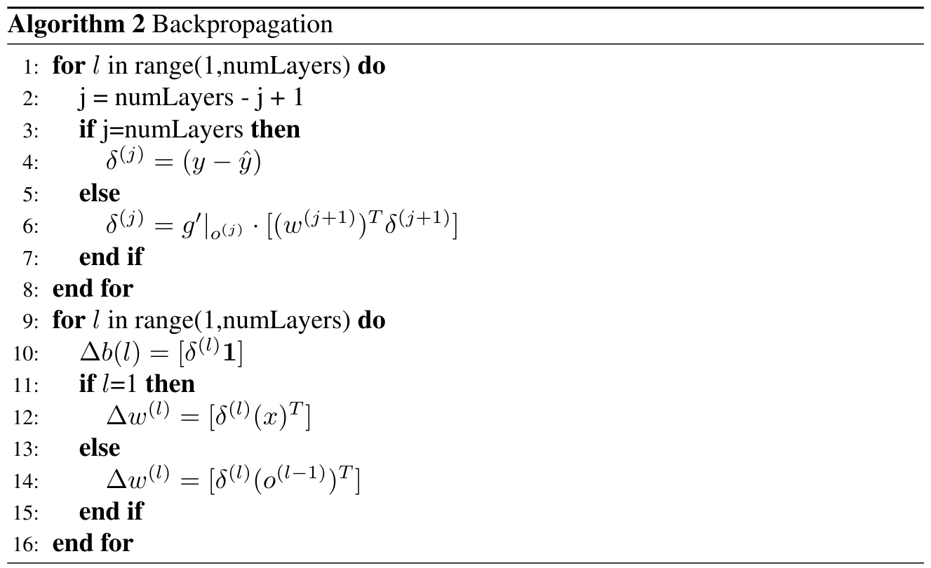
In this figure, we have a policy represented by $\pi$ and parameterized by $\theta$, and an approximate posterior represented by $q$ and parameterized by $\phi$. We start with a set of person-specific embeddings initialized uniformly. As training proceeds, we infer the person-specific embeddings ($\omega$ is a learned latent encoding via gradient descent) and learn a policy representing all demonstrators. We display a sample algorithm in Figure 4 for learning $\theta$, $\phi$, and $\omega$.

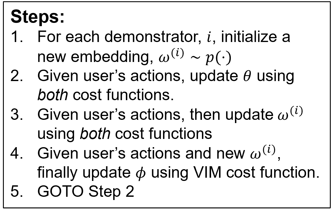
In step 1 of the algorithm, we sample from the set of demonstrators and obtain the trajectories associated with the sampled demonstrator. We initialize a new embedding, $\omega^{(i)}$, for the demonstrator. In step 2 and 3, we conduct a forward pass through the architecture displayed in Figure 3 and update parameters $\theta$ and $\omega$ via both the behavior cloning and VIM loss. In step 4, we utilize the VIM cost function to update $\phi$. We repeat this process until convergence. Once the algorithm has converged, every demonstrator’s person-specific embedding will accurately represent their modality. Utilizing this latent embedding within the learned policy will produce a representation of the demonstrator’s behavior.

In conclusion, the main takeaways from our blog post are as follows:

1. It is important to model the heterogeneity when Learning from Heterogeneous Demonstration (LfHD). We present a framework that can adapt to a person’s unique characteristics while simultaneously leveraging any homogeneity within the data.
2. We infer person-specific latent embeddings with semantic meaning by maximizing the lower bound of the mutual information between an inferred latent variable and a policy that is conditioned upon the latent variable.

Further Details

If you want to explore more on this, feel free to check our recent NeurIPS paper.

Previously, we covered gradient descent, an optimization method that adjusts the values of a set of parameters (e.g., the parameters of a linear regression model) to minimize a loss function (e.g., the mean squared error of a linear regression model network in predicting the value of a home given its zip code and other information). In this post, we introduce neural networks, which are essentially hyperparameter function approximators that learns to map a set of inputs to a set of outputs.

To optimize a neural network model with respect to a given loss function, we could directly apply gradient descent to adapt the parameters of a neural network to learn a desired mapping of inputs to outputs, this process would be inefficient. Due to the large number of parameters, performing symbolic differentiation as introduced in our gradient descent lesson would require a lot of redundant computation and slow down the optimization process tremendously. Fortunately, there is a better way: the backpropagation algorithm. Backpropagation is a form of auto-differentiation that allows us to more efficiently compute the derivatives of the neural network (or other model’s) outputs with respect to each of its parameters. Backpropagation is often overlooked or misunderstood as a simple application of symbolic differentiation (i.e., the chain rule from Calculus), but it is much, much more.

This blog will cover

1. Neural Networks
2. Forward Propagation
3. Backpropagation

We will not take the time to discuss the biological plausibility of neural networks, but feel free to check out this paper.

Neural Networks

We will start by understanding what a neural network is. At its core, a neural network is a function approximator. Functions from algebra, such as $y=x^2$ and $y=2x+1$, can be represented by neural networks. Neural networks can be used to learn a mapping given a set of data. For example, a neural network could be used to model the relationship of the age of a house, the number of bedrooms, and the square footage with the value of a house (displayed in Figure 1).

While the example in Figure 1 may appear trivial, neural networks can solve much more challenging problems. For example, neural networks have been applied to take as input Magnetic Resonance Imaging (MRI) data and output diagnoses for the patient based upon what is present in the MRI. Neural networks have also had success in being applied to problems of “machine translation” in which one attempts to translate one language to another (e.g., English to Chinese).

Typically, neural networks are given a dataset $\mathcal{D}=\{(x_k,y_k),\ k\in [n]\}$, where $(x_k,y_k)$ is the   “example” number $k$, $x_k$ is the input to a model we want to train, and $y_k$ is the “label” we want our model to learn to predict from $x_k$. We generalize the notation to $x$ being the input data, and $y$ being the set of ground-truth labels. A neural network can be represented as a function $\hat{y} = f(x)$ (i.e., $f: X \rightarrow Y$). Here, we use “$\hat{y}$” as the output of the neural network instead of “$y$,” as $\hat{y}$ is our estimate of the ground-truth label, $y$. Later, we will use the difference (i.e., error) between $\hat{y}$ and $y$, to optimize our neural network’s parameters.

If we look inside the function $f$, we see nodes and edges. These nodes and edges make up a directed graph, in which an input is operated on from left to right.

 

A closer look inside a smaller neural network is shown in Figure 2. Figure 2 displays how an input, $x$ (with cardinality $|x|=d$), is mapped to an output, $\hat{y}$, a scalar. Before we move into what is happening here, let’s will first explain the notation.

We have neural network weights, denoted by $w$, that weight the incoming value through multiplication. The subscripts represent the (to, from) nodes respectively, and the superscript denotes the layer number resulting in the notation as $w^{(layer)}_{to,from}$. The terms with the number “1” inside are termed bias nodes and are represented in the notation “b_{to}”.

As an example, we present a simple neural network describing $\hat{y} = 2x + 4z +3$ in Figure 4.

When an input is passed into a neural network, the input $x$ is multiplied by respective weights (denoted by $w$) and added to by a bias term $b$, resulting in a new value represented within a hidden node. In our model, we set the number of nodes in each layer to $n$. Each node, along with its incoming edges, represents some inner function. As our neural network can have many nodes and many layers, neural networks can be thought of as a composition of these inner functions to produce a more complex, outer function $f$ described above. The backslash in the most-right node represents a summation, resulting in a scalar value output. Now we will discuss precisely how to produce an output $\hat{y}$ given an input $x$ through learning a mapping.

Forward Propagation

The final output $\hat{y}$ is computed from the node values and weights of the previous layer, in our case, layer 2. We can multiply the output of the hidden nodes in layer 2, denoted by $o^{(2)}_i$, where $i$ represents a node index from $i$ to $n$ (i.e., $i \in \{1,2,\ldots,n\}$, by the weights connecting these nodes with the output node and add the bias term b^{(3)}_{i}. We display this process in Equation 1.

\begin{align}
\hat{y} = \sum_{i=1}^n w_{1,i}^{(3)} o^{(2)}_i + b^{(3)}_{1}
\end{align}

But, what is $o_i^{(2)}$ equal to? We display how $o_i^{(2)}$ is computed in Equation 2.

\begin{align}
o_i^{(2)} = g(z_i^{(2)})
\end{align}

Here, $i$ is again the node index and $g$ is an activation function (i.e., $g: Z \rightarrow O$). Neural networks cannot represent nonlinear functions without utilizing nonlinear activation functions. Activation functions help neural networks represent more complex functions by transforming node values by a nonlinear function. Common activation functions used include ReLU, tanh, sigmoid, etc. Here, we will discuss and use the ReLU (Rectified Linear Unit) as our activation function.

For our example, we will use the ReLU activation function, as shown in Equation 3.

\begin{equation}g(z) =\bigg\{\begin{aligned} &z \text{ if }z \geq 0\\ &0 \text{ otherwise}\end{aligned}\bigg\}\end{equation}

It is also helpful to know the gradient of the ReLU function, displayed in Equation 4.

\begin{equation}g'(z) =\bigg\{\begin{aligned} &1 \text{ if }z \geq 0\\ &0 \text{ otherwise}\end{aligned}\bigg\}\end{equation}

Moving back to Equation 2, we solve for $z_i^{(2)}$ in Equation 5.

\begin{align}
z^{(2)}_i = \sum_{j=1}^n w_{i,j}^{(2)} o^{(1)}_j + b^{(2)}_{i}
\end{align}

This procedure can be used throughout the neural network, computing the current layer using the previous layer’s output. For simplicity of algorithmic notation, you can consider the neural network’s input, $x$, as $o^{(0)}$. Here, $o^{(0)}$ represents the hypothetical output of a hypothetical zeroth layer. In Algorithm 1, we display the complete forward propagation algorithm, expressing the layer number as a variable for generalizability. This algorithm computes a predicted output, represented by $\hat{y}$, given input features, $x$.

We can now analyze the computational complexity of this algorithm. For the sake of simplifying the analysis, we assume the number of layers in the neural network, $l$, is equal to the number of nodes in each layer, $n$, which we also set as equal to the size of the input, $|x|=d$. Thus, $n=l=w$. In Algorithm 1, Steps 3 and 5 represent a matrix multiplication combined with addition. This process has a complexity of $O(n^2+n)$. As a reminder, for any matrix multiplication of two matrices of size $p \times q$ and $q \times r$, respectively, the computational complexity of this multiplication is $O(pqr)$. Thus, since we are multiplying weight matrices of size $n \times n$ to a vector of size $n \times 1$, the complexity of the matrix multiplication alone is $O(n \times n \times 1) = O(n^2)$. The addition operation adds complexity $O(n)$, resulting in $O(n^2+n)$ for Steps 2-6. Steps 8-10 have a complexity of $O(n)$ leading, resulting now in the complexity $O(n^2 + 2n)$. Since Step 1 iterates $n=l$ times, we arrive at a total complexity of $O(n(n^2 + 2n))=O(n^3)$ for Algorithm 1.

Now that we can perform a forward pass and know its complexity, we can discuss how to update our weights and attempt to learn a model that fits the data.

Backpropagation

To optimize our neural network weights to more accurately represent our data, we first establish a loss function that quantifies our model’s error (i.e., how wrong its outputs are for a desired task). Given this loss function, we could then compute the gradients of our loss function with respect to each weight. We could then perform gradient descent to optimize our model parameters as we did in the gradient descent blog post. However, we will now do something a bit more sophisticated to make the optimization process more computationally efficient.

Let’s consider a common loss function, as shown in Equation 6. This loss function represents a mean-squared error loss between the true label (true y-value in the data) and the predicted value using our neural network ($\hat{y}$).

\begin{align}
L=\frac{1}{2} (y-\hat{y})^2 = \frac{1}{2} (y-f(x))^2
\end{align}

The derivative of this loss function with respect to $w_{1,1}^{(1)}$ is displayed in Equation 7 according to chain rule.

\begin{align}
\frac{\partial L}{\partial w_{1,1}^{(1)}} = (y-\hat{y}) * \frac{\partial \hat{y}}{\partial w_{1,1}^{(1)}} \bigg|_x
\end{align}

So, how do we comput $\frac{\partial \hat{y}}{\partial w_{1,1}^{(1)}}$? There are 4 paths from the output node to $w_{1,1}^{(1)}$, which highlighted in blue in Figure 4. The upper-most path has the gradient shown in Equation 8.

\begin{align}
\frac{\partial \hat{y}}{\partial w_{1,1}^{(1)}} =  \frac{\partial \hat{y}}{\partial o^{(3)}} \frac{\partial o^{(3)}}{\partial z^{(3)}} \frac{\partial z^{(3)}}{\partial o^{(2)}_1} \frac{\partial o^{(2)}_1}{\partial z^{(2)}_1} \frac{\partial z^{(2)}_1}{\partial o^{(1)}_1} \frac{\partial o^{(1)}_1}{\partial w_{1,1}^{(1)}}
\end{align}

The rule for computing the “total derivative” encompassing all of these paths can be seen through an example here.

Computing a single partial derivative is computationally expensive, and computing each weight’s partial derivative individually (e.g., (e.g., $\frac{\partial \hat{y}}{\partial w_{1,1}^{(1)}}$ and then $\frac{\partial \hat{y}}{\partial w_{1,2}^{(1)}}$) and so forth all the way to $\frac{\partial \hat{y}}{\partial w_{1,n}^{(l)}}$) would be terribly inneficient.

If we instead look at $\frac{\partial \hat{y}}{\partial w_{1,2}^{(1)}}$, you can see that it shares many of the same nodes as $\frac{\partial \hat{y}}{\partial w_{1,1}^{(1)}}$. In Figure 5, we display a depiction of gradient computations required for $w_{1,1}^{(1)}$, $w_{2,1}^{(1)}$, and the overlap in the computations.

We would like to take advantage of this overlap in computation, which is exactly where the Backpropagation algorithm comes in. Backpropagation is a form of reverse-mode automatic differentiation that allows us to eliminate redundant computation in applying the chain rule to compute the gradient of our neural network.

Applied to neural networks, the backpropagation algorithm starts from the last layer of the neural network, computes an error term (denoted as $\delta$), and multiplies this error term by the gradient. The algorithm computes each node’s respective gradient in memory and reuses these variables as the algorithm continues, backpropagating the information for efficiency. We display the algorithm for Backpropagation in Algorithm 2. The output of the Backpropagation algorithm is gradients for each set of weights and biases.

Looking at the computational complexity of this algorithm, we see Step 4 has a complexity of $O(1)$. Step 6 has a complexity of $O(n^2 + n)$ or $O(n^2)$. Step 10 has a complexity of $O(n)$. Steps 12 and 14 both have complexities of $O(n^2)$. Since we iterate over the number of layers, equal to $n$ for our analysis, the total complexity is $O(n^3)$. If we did not use the Backpropagation algorithm, we would end up redundantly computing each component’s derivatives multiple times. Using the previous assumptions setting the cardinality of $|x|$, the number of nodes, and the number of layers to $n$, we would be iterating over $O(n^3 + n^2)$ weight derivatives resulting in a total complexity of $O(n^6)$.

The last step in optimizing our neural network model to minimize our loss function is to update weights and biases. Equations 9-10 show one step of gradient descent using the derivatives from our backpropagation procedure in Algorithm 2. Note that Equations 9-10 represent only one step of gradient descent, so one would need to iteratively perform the forward pass, then backward pass, then parameter updates (Equations 9-10) until the model converges to a local minimum, as described in our previous post on gradient descent.

\begin{align}
w^{(l)} \to w^{(l)} + \alpha \Delta w^{(l)}
\end{align}
\begin{align}
b^{(l)} \to b^{(l)} + \alpha \Delta b^{(l)}
\end{align}

We now have the ability to train neural networks in a computationally efficient manner, which, in turn, allows us to do more training iterations per unit time, which should help us train more accurate neural networks!

Key Points throughout this Blog:

1. Neural networks can be used to represent almost any function.
2. Forward propagation is the process of taking input features, $x$, and computing an output in the form of a model’s estimate, $\hat{y}$.
3. We can use the difference in the output, $\hat{y}$, of the neural network and our ground-truth data, $y$, to compute a loss, and then use this loss value to compute gradients in the backpropagation algorithm.
4. Backpropagation is a special case of reverse-mode automatic differentiation and allows for efficient gradient computation. The result is that the training of extremely large neural networks is possible!

In our previous blog post on Value Iteration & Q-learning, we introduced the Markov Decision Process (MDP) as a helpful model for describing the world, and we described how a robot could apply Reinforcement Learning (RL) techniques to learn a policy, $\pi: S \rightarrow A$, that maps the state of the world, $s \in S$, to the action the robot should take, $a \in A$. The goal of RL is to learn the optimal policy, $\pi^*$, that maximizes the expected, future, discounted reward (or return), $V^{\pi}(s)$, the agent receives when starting in state, $s$, and following policy, $\pi$ as given by the equation below.

\begin{align}
\pi^* = \text{arg}\max\limits_{\pi \in \Pi} V^{\pi}(s) = \text{arg}\max\limits_{\pi \in \Pi} \sum\limits_{s’}T(s,\pi(s),s’)[R(s,\pi(a|s),s’) + \gamma V_{\pi}(s’)]
\end{align}

We note that, in the tabular setting (e.g., for value and policy iteration, where one uses a look-up table to store information), the policy is deterministic (i.e, $\pi: S \rightarrow A$). However, when we move to deep learning-based representations of the policy (see the section on Policy Gradient below), the policy typically represents a policy distribution over actions the robot would sample from for acting in the world (i.e., $\pi: S \rightarrow [0,1]^{|A|}$).

To find the optimal policy, we described two approaches in our previous post (i.e., Value Iteration & Q-learning). Value iteration computes the optimal value function, $V^{*}(s)$, from which one can find the optimal policy given by $\pi^*(s) = \text{arg}\max\limits_{a \in A} \sum\limits_{s’}T(s,a,s’)[R(s,\pi(a|s),s’) + \gamma V^{*}(s’)]$. We also introduced Q-learning, in which one can extract the optimal policy by $\pi^*(s) = \text{arg}\max\limits_{a \in A} Q^*(s,a)$, where $Q^*$ is the optimal Q-function. Finally, we extended Q-learning to Deep Q-learning where the Q-function is represented as a neural network rather than storing the Q-values for each state-action pair in a look-up table.

In this blog post, we will follow a similar procedure for two new concepts: (1) Policy Iteration and (2) Policy Gradients (and REINFORCE). Like value iteration, policy iteration is a tabular method for reinforcement learning. Similar to Deep Q-learning, policy gradients are a function approximation-based RL method.

Policy Iteration

The pseudocode for policy iteration is given in Figure 1. At a high level, this algorithm first initializes a value function, $V(s)$, and a policy, $\pi(s)$, which are almost surely incorrect. That’s okay! The next two steps, (2) Policy Evaluation and (3) Policy Improvement, work by iteratively correcting the value function given the policy, correcting the policy given the value function, correcting the value function given the policy, and so forth. Let’s break down the policy evaluation and policy improvement steps.

Policy Evaluation

Policy evaluation involves computing the value function, $V^{\pi}(s)$, which we know how to do from our previous lesson on value iteration.
\begin{align}
V^\pi(s) = \sum\limits_{s’}T(s,\pi(s),s’)[R(s,\pi(s),s’) + \gamma V_{\pi}(s’)]
\end{align}

In policy iteration, the initial value function is chosen arbitrarily, (can be all zeroes, except at the terminal state – which will be the episode reward), and each successive approximation is computed using the following update rule:
\begin{align}
V_{k+1}(s) \: = \: \sum\limits_{s’}T(s,\pi(s),s’)[R(s,\pi(a|s),s’) + \gamma V_{k}(s’)]
\label{Bellman}
\end{align}

We keep updating the value function for the current policy using equation \ref{Bellman} until it converges (i.e., no state value is updated more than $\Delta$ during the previous iteration.

A key benefit of the policy evaluation step is that the DO-WHILE loop can exactly be solved as a linear program (LP)! We do not actually need to use dynamic programming to iteratively estimate the value function! Linear programs are incredibly fast, enabling us to quickly, efficiently find the value of our current policy. We contrast this ability with Value Iteration in which a $\max$ operator is required in the equation $V(s) = \text{arg}\max\limits_{a \in A} \sum\limits_{s’}T(s,a,s’)[R(s,a,s’) + \gamma V_{\pi}(s’)]$, which is nonlinear. Thus, we have identified one nice benefit of policy iteration already!

Policy Improvement

In the policy evaluation step, we determine the value of our current policy. With this value, we can then improve our policy.

Suppose we have determined the value function $V_\pi$ for a suboptimal, deterministic policy, $\pi$. By definition, then, the value taking the optimal action in a given state, $s$, would be at least as good if not better than the value of taking the action dictated by $\pi$. This inequality is given by:

\begin{align}
V^{\pi}(s) = \sum\limits_{s’}T(s,\pi(a|s),s’)[R(s,\pi(s),s’) + \gamma V^{\pi} (s’)] \leq \text{arg}\max\limits_{a \in A} \sum\limits_{s’}T(s,\pi(a|s),s’)[R(s,\pi(s),s’) + \gamma V^{\pi} (s’)], \forall s \in S
\end{align}

Thus, we should be able to find a better policy, $\pi'(s)$, by simply setting choosing the best action as given by the value function, $V^{\pi}(s)$ for our suboptimal policy, $\pi$, as given by:

\begin{align}
\pi'(s)  \leftarrow \text{arg}\max\limits_{a \in A} \sum\limits_{s’} T(s’,a,s) [R(s,a,s’) + \gamma V(s’)]
\end{align}

Thus, we can replace $\pi$ with $\pi’$, and we are done improving our policy until we have a new value function estimate (i.e., by repeating the Policy Evaluation Step). The process of repeatedly computing the value function and improving policies starting from an initial policy $\pi$ (until convergence) describes policy iteration.

Just like how Value Iteration & Q-learning have their deep learning counterparts, so does our Policy Iteration algorithm.

Policy Gradient

As explained above, RL seeks to find a policy, $\pi$, that maximizes the expected, discounted, future reward given by following the actions dictated by policy, $\pi(s)$ in each state, $s$. In Policy Iteration, we first compute the value, $V^{\pi}(s)$, of each state and use these value estimates to improve the policy, $\pi$. Let $\theta$ denote the policy parameters of a neural network. We denote this policy as $\pi_{\theta}(s)$. Unlike the policy iteration method, policy gradient methods learn a parameterized policy (commonly parameterized by a neural network) to choose actions without having to rely on a table to store state-action pairs (and, arguably, without having to rely on an explicit value function; however, that depends on your formulation, which we will return to later).

With policy gradients, we seek to find the parameters, $\theta$, that maximizes the expected future reward. Hence, policy gradient methods can be formulated as a maximization problem with the objective function being the expected future reward as depicted in Equation \ref{PG_obj}, where $V^{\pi_\theta}$ is the value function for policy parameterized by $\theta$.
\begin{align}
J(\theta) \: =  \mathbb{E}_{s \sim \rho(\cdot)} V^{\pi_\theta}(s) = \mathbb{E}_{s \sim \rho(\cdot), a \sim \pi(s)} \left[\sum\limits_{t=0}^\infty \gamma^t r_{t} | s_0 = s\right]
\label{PG_obj}
\end{align}

To maximize $J(\theta)$, we perform gradient ascent as shown in Equation \ref{gradient ascent}. For more details on solving optimization problems with gradient-based approaches, please see the blog post on Gradient Descent.
\begin{align}
\theta_{k+1} = \theta_k + \alpha \nabla_\theta J(\theta)
\label{gradient ascent}
\end{align}

In the case of policy gradient methods, the action probabilities change smoothly as a function of the learned parameters, $\theta$, whereas in tabular methods (e.g., Policy Iteration), the actions may change drastically even for small changes in action value function estimates. Thus, policy gradient-based methods may be more sample-efficient when this assumption holds by essentially interpolating the right action when in a new state (or interpolating the right Q-value in the case of Q-learning). However, if this smoothness property does not hold, neural network function approximation-based RL methods, e.g., Deep Q-learning or Policy Gradients, will struggle. Nonetheless, this smoothness assumption does commonly hold — at least enough — that deep learning-based methods are the mainstay of modern RL.

The Policy Gradient Theorem

(This derivation is adapted from Reinforcement Learning by Sutton & Barto)

We will now compute the gradient of the objective function $J(\theta)$ with respect to the policy parameter $\theta$. Henceforth, we will assume that the discount factor, $\gamma=1$, and $\pi$ in the derivation below represents a policy parameterized by $\theta$.
\begin{align}
\begin{split}
\nabla_\theta J(\theta) &= \nabla_\theta(V_{\pi_\theta}) \\
&= \nabla_\theta \left[\sum\limits_a \pi_\theta(a|s) Q_{\pi}(s,a)\right] \; \; \; \; \; \; \; \; \; \; \; \; \; \; \; \; \; \; \; \; \; \; \; \; \; \; \; \; \; \; \; \; \; \; \; \; \; \; \; \; \; \; \; \; \; \; \; \; \; \; \; \; \; \; \; \; \; \; \; \; \; \; \; \; \; \; \; \; \; \; \; \; \; \; \; \; \; \; \; \; \; \; \; \; \; \; \; \; \text{(From }\ref{Q_v})\\
&= \sum\limits_a \Bigg[\nabla_\theta \pi_\theta(a|s) Q_{\pi}(s,a) + \pi_\theta(a|s) \nabla_\theta Q_{\pi}(s,a) \Bigg] \; \; \; \; \; \; \; \; \; \; \; \; \; \; \; \; \; \; \; \; \; \; \; \; \; \; \; \; \; \; \; \; \; \; \; \; \; \; \; \; \; \; \; \; \; \; \; \; \; \; \; \; \; \; \; \; \; \text{(by product rule)}\\
&= \sum\limits_a \Bigg[\nabla_\theta \pi_\theta(a|s) Q_{\pi}(s,a) + \pi_\theta(a|s) \nabla_\theta \left[\sum\limits_{s’} T(s,a,s’)[R(s,a,s’) + V_{\pi}(s’)] \right]\Bigg]\\
&= \sum\limits_a \Bigg[\nabla_\theta \pi_\theta(a|s) Q_{\pi}(s,a) + \pi_\theta(a|s) \sum\limits_{s’} T(s,a,s’)\nabla_\theta V_{\pi}(s’) \Bigg]\\
\text{Unrolling $V_{\pi}(s’)$, we have… }\\
&= \sum\limits_a \Bigg[\nabla_\theta \pi_\theta(a|s) Q_{\pi}(s,a) + \pi_\theta(a|s) \sum\limits_{s’} T(s,a,s’) \sum\limits_{a’} \Bigg[\nabla_\theta \pi(a’|s’)Q_{\pi}(s’,a’) + \pi(a’|s’)\sum\limits_{s'{}’} T(s’,a’,s'{}’) \nabla_\theta V_{\pi}(s'{}’) \Bigg] \Bigg]\\
\end{split}
\end{align}
We can continue to unroll $V_{\pi}(s'{}’)$ and so on…Unrolling ad infinitum, we can see:
\begin{align}
\nabla_\theta J(\theta) \: = \: \sum\limits_{s \in \mathcal{S}} \sum\limits_{k=0}^{\infty}Pr(s_0 \rightarrow s, k, \pi)\sum\limits_a \nabla_\theta \pi_\theta(a|s) Q_\pi(s,a)
\label{PG_1}
\end{align}
Here, $Pr(s_0 \rightarrow s, k, \pi)$ is the probability of transitioning from state $s_0$ to $s$ in $k$ steps while following the policy $\pi$. Rewriting $Pr(s_0 \rightarrow s, k, \pi)$ as $\eta(s)$ in Equation \ref{PG_1}, we have:
\begin{align}
\begin{split}
\nabla_\theta J(\theta) \: &= \: \sum\limits_{s} \eta(s)\sum\limits_a \nabla_\theta \pi_\theta(a|s) Q_\pi(s,a)\\
&= \: \sum\limits_{s’} \eta(s’) \sum\limits_{s} \frac{\eta(s)}{\sum\limits_{s’}\eta(s’)} \sum\limits_a \nabla_\theta \pi_\theta(a|s) Q_\pi(s,a)\\
&= \: \sum\limits_{s’} \eta(s’) \sum\limits_{s} \mu(s) \sum\limits_a \nabla_\theta \pi_\theta(a|s) Q_\pi(s,a)\\
&\propto \: \sum\limits_{s} \mu(s) \sum\limits_a \nabla_\theta \pi_\theta(a|s) Q_\pi(s,a)\\
\end{split}
\label{PG_final}
\end{align}

We note that we set $\mu(s) = \frac{\eta(s)}{\sum\limits_{s’}\eta(s’)}$ for convenience. Now, one might ask, what about the derivation for $\gamma \neq 1$? Well, that is a great question! Candidly, we have not seen a clean derivation when $\gamma \in (0,1)$, and we would welcome any readers out there to email us should such a derivation exist that we could link to!

REINFORCE – Monte Carlo Policy Gradient

From Equation \ref{PG_final}, we find an expression proportional to the gradient. Taking a closer look at the right-hand side of Equation \ref{PG_final}, we note that it is a summation over all states, weighted by how often these states are encountered under policy $\pi$. Thus, we can re-write Equation \ref{PG_final} as an expectation:
\begin{align}
\begin{split}
\nabla_\theta J(\theta) \: &\propto \: \sum\limits_{s} \mu(s) \sum\limits_a \nabla_\theta \pi_\theta(a|s) Q_\pi(s,a)\\
&= \: \mathbb{E}_{s \sim \mu(\cdot)}\left[\sum\limits_a \nabla_\theta \pi_\theta(a|s) Q_\pi(s,a) \right] \\
\end{split}
\label{PG_grad}
\end{align}
We modify the gradient expression in Equation \ref{PG_grad} by (1) introducing an additional weighting factor $\pi_\theta(a|s)$ and dividing by the same without changing the equality, and (2) sampling an action from the distribution instead of summing over all actions. The modified update rule for the policy gradient algorithm is shown in Equation \ref{REINFORCE}.
\begin{align}
\begin{split}
\nabla_\theta J(\theta)\: &= \: \mathbb{E}_{s \sim \mu(\cdot)}\left[\sum\limits_a \pi_\theta(a|s) Q_\pi(s,a) \frac{\nabla_\theta \pi(a|s)}{\pi(a|s)} \right] \\
&= \: \mathbb{E}_{s \sim \mu(\cdot), a\sim \pi(\cdot|s)}\left[Q_\pi(s,a) \frac{\nabla_\theta \pi_\theta(a|s)}{\pi_\theta(a|s)} \right] \; \; \; \; \; \; \; \; \; \; \; \; \; \; \; \; \; \; \; \; \; \; \; \; \; \; \; \; \; \; \; \; \; \; \; \; \; \; \; \; \; \; \; \; \text{($a$ here is sampled from $\pi$)}\\
&= \: \mathbb{E}_{s \sim \mu(\cdot), a\sim \pi(\cdot|s)}\left[Q_\pi(s,a) \nabla_\theta \: \text{log}\: \: \pi_\theta(a|s) \right] \; \; \; \; \; \; \; \; \; \; \; \; \; \; \; \; \; \; \; \; \; \; \; \; \; \; \; \; \; \; \; \; \; \; \; \; \; \; \; \left(\nabla_\theta \: \text{log}\: \: \pi_\theta(a|s) = \frac{\nabla_\theta \pi_\theta(a|s)}{\pi_\theta(a|s)} \right)\\
&= \: \mathbb{E}_{s \sim \mu(\cdot), a\sim \pi(\cdot|s)}\left[G_t \nabla_\theta \: \text{log}\: \: \pi_\theta(a|s) \right] \; \; \; \; \; \; \; \; \; \; \; \; \; \; \; \; \; \; \; \; \; \; \; \; \; \; \; \; \; \; \; \; \; \; \; \; \; \; \; \; \; \; \; \; \; \; \; \; \; \text{($G_t$ is the return, and $\mathbb{E}_{\pi}[G_t|S_t=s, A_t=a] = Q_\pi(s,a)$)}\\
\end{split}
\label{REINFORCE}
\end{align}
Including the logarithm creates a weighting factor based on the probability of occurrence of different state-action pairs, allowing us to leverage the expected gradient update over actions without numerically estimating the expectation! The final expression within the expectation in Equation \ref{REINFORCE}, is the quantity that can be sampled at each timestep to update the gradient. The REINFORCE update using gradient ascent is described in Equation \ref{grad_update}.
\begin{align}
\theta_{t+1} \: \dot{=} \: \theta_t + \alpha G_t \: \nabla_{\theta} \: \text{log}\: \: \pi_{\theta_t}(a|s)
\label{grad_update}
\end{align}

Fig. 2 shows the complete REINFORCE algorithm.

Returning to our aside from earlier about whether policy gradients rely on an estimate of the value function, our derivation here, as depicted in Fig. 2, does not rely on the value function. However, as our derivation alluded to, one could use the value function for $G_t = V^{\pi}(s)$. One could also use the Q-function, $G_t = Q^{\pi}(s,a)$. When setting $G$ equal to the value or Q-function, we refer to the the update as a actor-critic (AC) method. When we use the advantage function formulation, $G_t = Q^{\pi}(s,a) – V^{\pi}(s)$, the update is known as an advantage function, actor-critic (A2C) method. For AC and A2C, we need neural network function approximators to estimate the Q- and/or value functions. While adding on and learning from these additional neural networks adds computational complexity, AC and A2C often work better in practice than REINFORCE. However, that is a point that we will leave for a future blog!

Takeaways

• A policy is a mapping from states to probabilities of selecting every possible action in that state. A policy $\pi^*$ is said to be optimal if its expected return is greater than or equal to any other policy $\pi$ for all states.
• Policy Iteration is a non-parametric (i.e., tabular, exact, not deep learning-based) approach to compute the optimal policy. Policy iteration alternates between policy evaluation (computing the value function given a policy) and policy improvement (given a value function) to converge to the optimal policy.
• Policy gradients are a powerful, deep learning-based approach to learning an optimal policy with neural network function approximation for the policy.

References

Richard S. Sutton and Andrew G. Barto. 2018. Reinforcement Learning: An Introduction. A Bradford Book, Cambridge, MA, USA.

Gradient Descent (GD) is an intuitive optimization method. GD has become one of the most popular optimization methods in recent years due to its nice theoretical properties, effectiveness in real-world applications, and uncanny ability to train large-scale deep learning models. GD is commonly used in deep learning for finding neural network parameters that best capture patterns in the data. In this blog, we introduce three different flavors of GD, regular GD, Stochastic GD (SGD), and Minibatch GD (MbGD). We analyze these variants theoretically as well as empirically, and discuss which one is most appropriate for different scenarios! Finally, we discuss how GD can be improved or “accelerated” by adding “momentum”.

This blog is divided into four parts:

1. Introduction of GD, SGD, and MbGD
2. Analytical results
3. Empirical results
4. Accelerated GD

What is GD, SGD, and MbGD?

Let’s first look at a simple machine learning scenario. We have a dataset $\mathcal{D}=\{(x_i,y_i),\ i\in [n]\}$, where $(x_i,y_i)$ is  “example” number $i$, $x_i$ is the input to a model we want to train and $y_i$ is the “label” we want our model to learn to predict from $x_i$. For instance, $x_i$ might be the date of the year, and $y_i$ might be the expected rainfall you would receive that day. In this simplified example, we assume $x_i$ is a scalar instead of a vector, but the concept and the math work for the vector case (where $x_i$ contains several features) too.

To allow us to visualize the model, let’s assume we are using a linear model parameterized by $\theta$ shown in Equation \ref{f}.
\begin{align}
f_\theta(x_i)=\theta x_i
\label{f}
\end{align}
The metric we use to judge our model (i.e., a “loss function”) is the Mean Squared Error (MSE) loss (Equation \ref{L}), which calculates the squared error for each prediction and averages over all data points.
\begin{align}
L(\theta)=-\frac{1}{2n}\sum_{i=1}^n(y_i-f_\theta(x_i))^2
\label{L}
\end{align}
We want to find the best model, $\theta^*$, according to our loss function (Equation \ref{loss}).
\begin{align}
\theta^*=\arg\min_\theta L(\theta)
\label{loss}
\end{align}

\(L\) is a quadratic function of the model parameter \(\theta\), illustrated in Figure 1. The problem then is to find the critical point, $\theta^*$, that is located at the minimum of this curve. To find the critical point, we set the first derivative of $L$ equals to $0$, i.e. $\frac{\partial L(\theta)}{\partial \theta}=0$. In the case of a simple linear model, we can directly solve for model parameters $\theta^*$. However, in deep learning, such direct methods do not exist. Instead, we need something else. In this tutorial, that “something else” is GD.

GD

In GD, we perform three steps:

1. Calculate the gradient of our model parameters.
2. Use the gradient to update model parameters.
3. Repeat steps 1 and 2 until a pre-set tolerance is achieved.

We use $\nabla$ as the gradient operator and it is defined in Equation \ref{gradient}.
\begin{align}
\nabla_\theta=\left[\begin{matrix}
\frac{\partial}{\partial \theta_1}\\
\frac{\partial}{\partial \theta_2}\\
\cdots\\
\frac{\partial}{\partial \theta_m}\\
\end{matrix}\right]
\label{gradient}
\end{align}
First, we calculate the gradient of $L$ w.r.t. $\theta$ in MSE loss (Equation \ref{L}), shown in Equation \ref{gradient_of_L}.
\begin{align}
\nabla_\theta L=-\frac{1}{n}\sum_{i=1}^n(y_i-f_\theta(x_i))\nabla_\theta f_\theta(x_i)\bigg\rvert_{x_i}
\label{gradient_of_L}
\end{align}
In our case of linear model (Equation \ref{f}), we could write the gradient as in Equation \ref{L_linear}.
\begin{align}
\begin{split}
\nabla_\theta L&=-\frac{1}{n}\sum_{i=1}^n(y_i-\theta x_i)x_i\\
&=\frac{1}{n}\sum_{i=1}^nx_i^2\theta-\frac{1}{n}\sum_{i=1}^nx_iy_i
\end{split}
\label{L_linear}
\end{align}
The gradient $\nabla_\theta L$ is a linear function of $\theta$, as shown in Figure 2.

Second, we would like to use the calculated gradient to update our model parameters. As we want to minimize the loss function, GD follows the negative gradient direction. We update our parameters by this gradient multiplied by a small step size $\alpha$ (a hyperparameter), as shown in Equation \ref{negative_gradient_step}.
\begin{align}
\theta^{(i)}\leftarrow \theta^{(i-1)}-\alpha \nabla_\theta L(\theta^{(i-1)})
\label{negative_gradient_step}
\end{align}
Empirically, we choose $\alpha$ to be ${10}^{-5}-{10}^{-3}$. Utilizing an $\alpha$ value that is too small will result in slower learning and require more iterations of (1) and (2). An $\alpha$ value that is too large may be even more detrimental. It may lead to behavior that causes the model parameters $\theta$ to oscillate or even diverge.

Finally, GD continues to iterate until a pre-set tolerance is achieved (norm of gradient is small, function value is small, or iteration number is large, etc).

If the function to be optimized (in our case, the loss function, $L$) is convex w.r.t. the parameters $\theta$, GD is guaranteed to converge to a global minimum given alpha is small enough. However, if this assumption does not hold, the model parameters could become stuck in a local minimum of the loss function $L$. For problems that are non-convex, we often perform GD several times with sets of randomly initialized theta, hoping to find the global minimum.

Why take the negative gradient direction?

In order to minimize the loss in Figure 1, we look at two cases: where $\theta >4.5$ and $\theta < 4.5$. If $\theta$ is greater than $4.5$, we need to move left along the loss curve to decrease our loss value. If $\theta$ is less than $4.5$, we should move right.

From Figure 2, we can see that $\nabla_\theta L>0$ when $\theta>4.5$ and $\nabla_\theta L <0$ when $\theta<4.5$. Utilizing the negative of these gradients in our update rules allows us to improve theta, i.e. decreases our loss function.

This idea of “taking a step” comes from using a first order Taylor Expansion of $L(\theta)$, mathematically shown in Equation \ref{taylor_expansion}.
\begin{align}
L(\theta^\prime)\approx L(\theta)+(\theta^\prime-\theta)\nabla_\theta L(\theta)
\label{taylor_expansion}
\end{align}
Therefore, if our goal is to make $L(\theta^\prime)$ smaller, we can take $\theta^\prime=\theta-\alpha\nabla_\theta L(\theta)$, as
\begin{align}
\begin{split}
L(\theta-\alpha\nabla_\theta L(\theta))&\approx L(\theta)-\alpha\nabla_\theta L(\theta)\nabla_\theta L(\theta) \\
&= L(\theta)-\alpha(\nabla_\theta L(\theta))^2\\
&< L(\theta).\quad ((\nabla_\theta L(\theta))^2\geq 0, \alpha>0)
\end{split}
\end{align}

Accordingly, GD is guaranteed to reduce the loss function if $\alpha$ is infinitely small. As a result, GD will go down the hill, as shown in Figure 1.

SGD

Stochastic Gradient Descent (SGD) has one fundamental difference compared to standard GD: instead of using the entire dataset to calculate the gradient $\nabla_\theta L$ in each step, we sample only one data point from the dataset and use that specific data to calculate $\nabla_\theta L$. Speficaly, in our example, the gradient of the loss function computed over one datapoint is shown in Equation \ref{gradient_SGD}.
\begin{align}
\begin{split}
\nabla_\theta L(\theta^{(i-1)})&=-(y_j-\theta^{(i-1)} x_j) x_j\\
&=x_j^2\theta^{(i-1)}-x_jy_j\\
& j\sim \mathcal{U}\{1,n\}
\end{split}
\label{gradient_SGD}
\end{align}
Here, $\mathcal{U}\{1,n\}$ represents discrete uniform distribution.

Because we only compute our gradient update for one data point, SGD requires less computation (Floating Point Operations Per Second, FLOPS) than GD in each iteration. However, since we are calculating the gradient from just one sample of data, and the data may be noise (typical in real-world datasets), SGD may take steps in the wrong direction.

MbGD

Minibatch Gradient Descent represents a middle ground between GD and SGD, sampling a small subset of examples from our dataset to calculate $\nabla_\theta L$:
\begin{align}
\begin{split}
\nabla_\theta L(\theta^{(i-1)})&=-\frac{1}{n^\prime}\sum_{j\in\mathcal{B^{(i)}}}(y_j-\theta^{(i-1)} x_j) x_j\\
&=\frac{1}{n^\prime}\sum_{j\in\mathcal{B^{(i)}}}x_j^2\theta^{(i-1)}-x_jy_j
\end{split}
\end{align}
In this equation, $\mathcal{B}=\{i_1,\cdots,i_{n^\prime}\}, i_j\sim \mathcal{U}\{1,n\}$. $n^\prime$ is the size of the minibatch. The size of minibatch is a hyperparameter you choose.

Visualization of GD, MbGD and SGD

The optimization process difference between the three variants of GD is illustrated in Figure 3. From GD to MBGD and SGD, the updating process becomes noisier and takes more iterations to converge. However, the computation time for each iteration is lower.

Comparison of Teoretical Properties

Here, we investigate the pros and cons for each gradient descent mechanism.

This table summarizes pros and cons of each GD variant.

	GD	MbGD	SGD
Noise in Updates	Low	Mid	High
FLOPS/iter	High	Mid	Low
RAM usage	High	Mid	Low

For large datasets such as Image-Net, it is impossible for GD to run on most computers as the memory requirement is extremely large (i.e., you cannot load the entire dataset, $\mathcal{D}$, into RAM).

We might wonder: since SGD only takes low FLOPS/iter but has high gradient noise, will it slow down SGD’s overall convergence?

Researchers have provided the answer (reference) ($k$ represents the algorithm iteration count):

This table displays the convergence rate of each GD variant under different assumptions.

	GD	SGD
Convex Function	$\mathcal{O}(\frac{1}{\sqrt{k}})$	$\mathcal{O}(\frac{1}{\sqrt{k}})$
Lipschitz Gradient + Convex Function	$\mathcal{O}(\frac{1}{k})$	$\mathcal{O}(\frac{1}{\sqrt{k}})$
Strongly Convex Function	$\mathcal{O}(\gamma^k)$	$\mathcal{O}(\frac{1}{k})$

Here, we measure convergence by $\mathbb{E}[L(\theta^{(k)})-L(\theta^*)]$ in which $\theta^*$ represents the best parameters.

Note that for a loss function $L$ to be convex, the second derivitve with respect to $\theta$ for ALL $\theta$ and $x_i\in \mathcal{D}$ must be positive (for differentible functions), as shown in Equation \ref{second_direvative_greater_than_0}.
\begin{align}
\frac{\partial^2 L(\theta)}{\partial \theta^2}\geq 0,\quad\forall\theta, x_i \in\mathcal{D}
\label{second_direvative_greater_than_0}
\end{align}
Performing GD on convex functions is guaranteed to find the global optimum, $\theta^*$. However, it is generally not guaranteed when functions are non-convex.

Lipschitz Gradient means the gradient of loss $L$ w.r.t. $\theta$ cannot change dramatically locally, as described in Equation \ref{lipschitz_gradient}.
\begin{align}
||\nabla L(\theta)-\nabla L(\theta^\prime)\leq \Omega ||\theta-\theta^\prime||,\quad\exists\Omega,\forall \theta,\theta^\prime
\label{lipschitz_gradient}
\end{align}

Strongly Convex means the function is not only convex but also has at least certain curvature as quadratic functions (reference), as shown in Equation \ref{strongly_convex}.
\begin{align}
\langle\nabla L(\theta)-\nabla L(\theta^\prime),\theta-\theta^\prime\rangle\geq \gamma ||\theta-\theta^\prime||^2,\quad\exists\gamma>0,\forall \theta,\theta^\prime
\label{strongly_convex}
\end{align}

Although these assumptions do not always hold for general loss functions and model choices, we can conclude that SGD’s convergence rate is not as good as GD in the latter two cases, but their convergence is actually the same under convex function assumption! In practice, we cannot say much about the theoretical properties of GD vs SGD, but we at least can go forward knowing that SGD performs comparably on convex functions and is often more feasible when working with Big Data.

Take Away

Although SGD seems to have more noisy updates, SGD’s convergence rate on convex function is the same as GD. Further, SGD requires fewer FLOPS/iter. Therefore, SGD would require fewer total FLOPS to find our best model, $\theta^*$. SGD for the win!

Empirical Comparison

Here, we show an example optimization of the three methods. In line with our theoretical results, they have similar convergence in terms of iterations, and GD > MbGD > SGD in terms of FLOPS.

Note that SGD does have higher noise during the process, and MbGD has similar smooth updates as GD, i.e., the usage of minibatch does help stabilize the update.

Take Away

When the dataset is small, GD is preferred due to its low-noise properties. When the dataset gets large enough, GD becomes infeasible. In this case, SGD is preferred if the data noise is not significant and the noisy updates will not ruin the optimization process, otherwise, MbGD is preferred. We provide our code on Github.

Accelerating GD and SGD

Several variants of GD (such as Momentum GD, RMSProp, Adam) all utilize the core idea of momentum. What is momentum then?

We introduce the initial momentum as
\begin{align}
m^{(0)}=0.
\end{align}

For each iteration, instead of using the gradient to directly update $\theta$, we use the gradient to update the momentum, as shown in Equation \ref{momentum}.
\begin{align}
m^{(i)}=\beta m^{(i-1)}+\nabla_\theta L(\theta^{(i-1)})
\label{momentum}
\end{align}
$\beta\in[0,1)$ is a hyperparameter that you tune, and $\beta=0$ recovers basic GD.
And then use the momentum to update $\theta$ according to Equation \ref{theta_update_momentum}.
\begin{align}
\theta^{(i)}=\theta^{(i-1)}-\alpha m^{(i)}
\label{theta_update_momentum}
\end{align}

What is momentum essentially doing, and when is it useful?

Consider the snowboarding-in-a-half-pipe-like optimization problem depicted in Figure 5.

Often in these situations, standard GD will oscillate back and forth because the gradient direction has larger value on vertical direction than horizontal direction. However, we could see that each gradient step still has a small right movement, slowly pushing us to the optimum.

Momentum techniques utilize such phenomenon and gathers the downward forces while canceling out the horizontal forces, resulting as the result shown before.

Another case that momentum helps is when the loss function has a flat region (plateau) as shown in Figure 7.

In this case, gradient descent updates on $\theta$ will get slower in the middle plateau area, even equaling $0$ in extreme cases. However, as long as we accumulate enough momentum before the plateau, we could rush over the plateau, avoiding the small-gradient problem. Momentum can also help push past local minimums so that we can find optimal parameters even if our function is non-convex.

Theoretically, it could be proven that a similar variant of Momentum GD, Nesterov’s accelerated gradient descent, could achieve $O(\frac{1}{k^2})$ convergence instead of $O(\frac{1}{k})$ (reference).

Take Away

Momentum is useful for solving many optimization problems. However, adding momentum in requires extra hyperparameter tuning for $\beta$.

Conclusion

1. GD, MbGD, SGD converge at the same rate in terms of iterations.
2. SGD requires fewer FLOPS but is noisy.
3. Parallization could help MbGD and GD do better in terms of wall clock time.
4. Momentum can help but needs careful hyperparameter tuning.
5. Many famous optimizers such as Adam use momentum and fancy tricks but it is essentially SGD!