Previously, we covered gradient descent, an optimization method that adjusts the values of a set of parameters (e.g., the parameters of a linear regression model) to minimize a loss function (e.g., the mean squared error of a linear regression model network in predicting the value of a home given its zip code and other information). In this post, we introduce neural networks, which are essentially hyperparameter function approximators that learns to map a set of inputs to a set of outputs.
To optimize a neural network model with respect to a given loss function, we could directly apply gradient descent to adapt the parameters of a neural network to learn a desired mapping of inputs to outputs, this process would be inefficient. Due to the large number of parameters, performing symbolic differentiation as introduced in our gradient descent lesson would require a lot of redundant computation and slow down the optimization process tremendously. Fortunately, there is a better way: the backpropagation algorithm. Backpropagation is a form of auto-differentiation that allows us to more efficiently compute the derivatives of the neural network (or other model’s) outputs with respect to each of its parameters. Backpropagation is often overlooked or misunderstood as a simple application of symbolic differentiation (i.e., the chain rule from Calculus), but it is much, much more.
This blog will cover
- Neural Networks
- Forward Propagation
- Backpropagation
We will not take the time to discuss the biological plausibility of neural networks, but feel free to check out this paper.
Neural Networks
We will start by understanding what a neural network is. At its core, a neural network is a function approximator. Functions from algebra, such as $y=x^2$ and $y=2x+1$, can be represented by neural networks. Neural networks can be used to learn a mapping given a set of data. For example, a neural network could be used to model the relationship of the age of a house, the number of bedrooms, and the square footage with the value of a house (displayed in Figure 1).
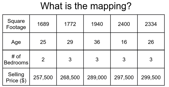
While the example in Figure 1 may appear trivial, neural networks can solve much more challenging problems. For example, neural networks have been applied to take as input Magnetic Resonance Imaging (MRI) data and output diagnoses for the patient based upon what is present in the MRI. Neural networks have also had success in being applied to problems of “machine translation” in which one attempts to translate one language to another (e.g., English to Chinese).
Typically, neural networks are given a dataset $\mathcal{D}=\{(x_k,y_k),\ k\in [n]\}$, where $(x_k,y_k)$ is the “example” number $k$, $x_k$ is the input to a model we want to train, and $y_k$ is the “label” we want our model to learn to predict from $x_k$. We generalize the notation to $x$ being the input data, and $y$ being the set of ground-truth labels. A neural network can be represented as a function $\hat{y} = f(x)$ (i.e., $f: X \rightarrow Y$). Here, we use “$\hat{y}$” as the output of the neural network instead of “$y$,” as $\hat{y}$ is our estimate of the ground-truth label, $y$. Later, we will use the difference (i.e., error) between $\hat{y}$ and $y$, to optimize our neural network’s parameters.
If we look inside the function $f$, we see nodes and edges. These nodes and edges make up a directed graph, in which an input is operated on from left to right.
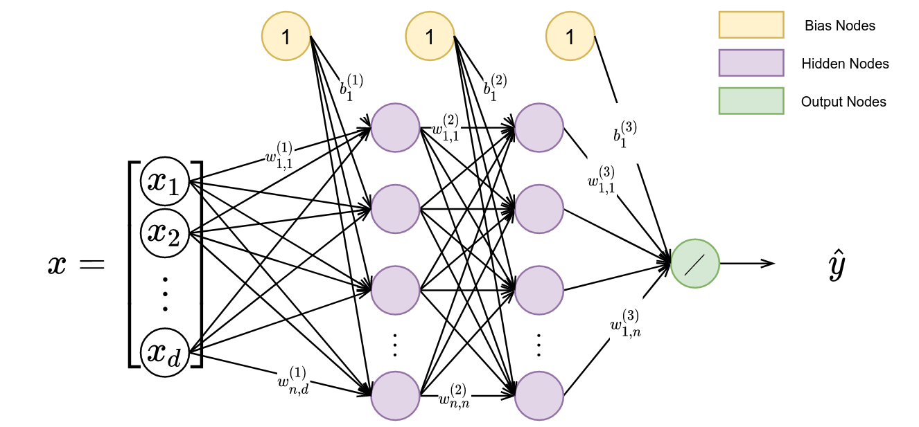
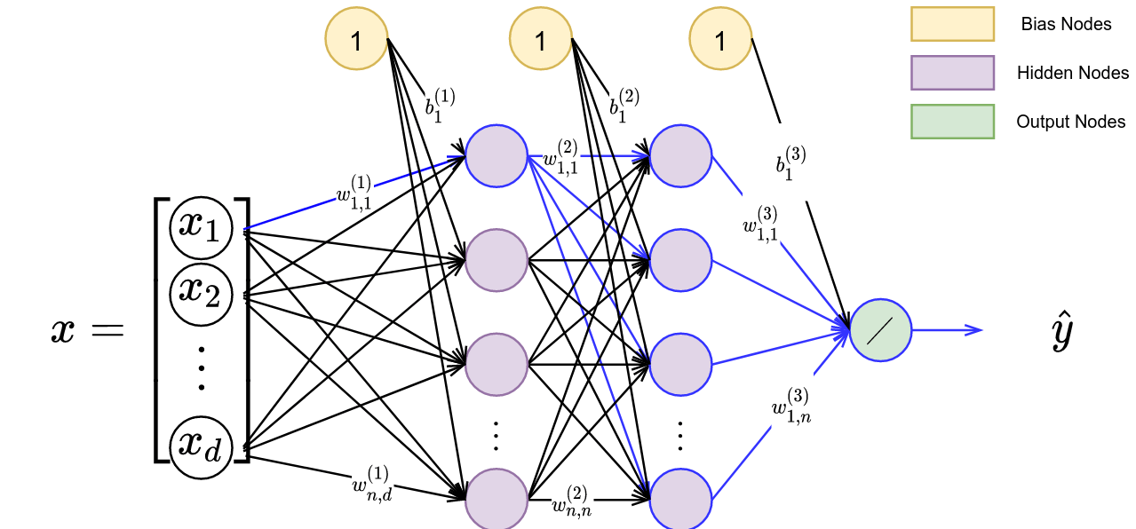
A closer look inside a smaller neural network is shown in Figure 2. Figure 2 displays how an input, $x$ (with cardinality $|x|=d$), is mapped to an output, $\hat{y}$, a scalar. Before we move into what is happening here, let’s will first explain the notation.
We have neural network weights, denoted by $w$, that weight the incoming value through multiplication. The subscripts represent the (to, from) nodes respectively, and the superscript denotes the layer number resulting in the notation as $w^{(layer)}_{to,from}$. The terms with the number “1” inside are termed bias nodes and are represented in the notation “b_{to}”.
As an example, we present a simple neural network describing $\hat{y} = 2x + 4z +3$ in Figure 4.
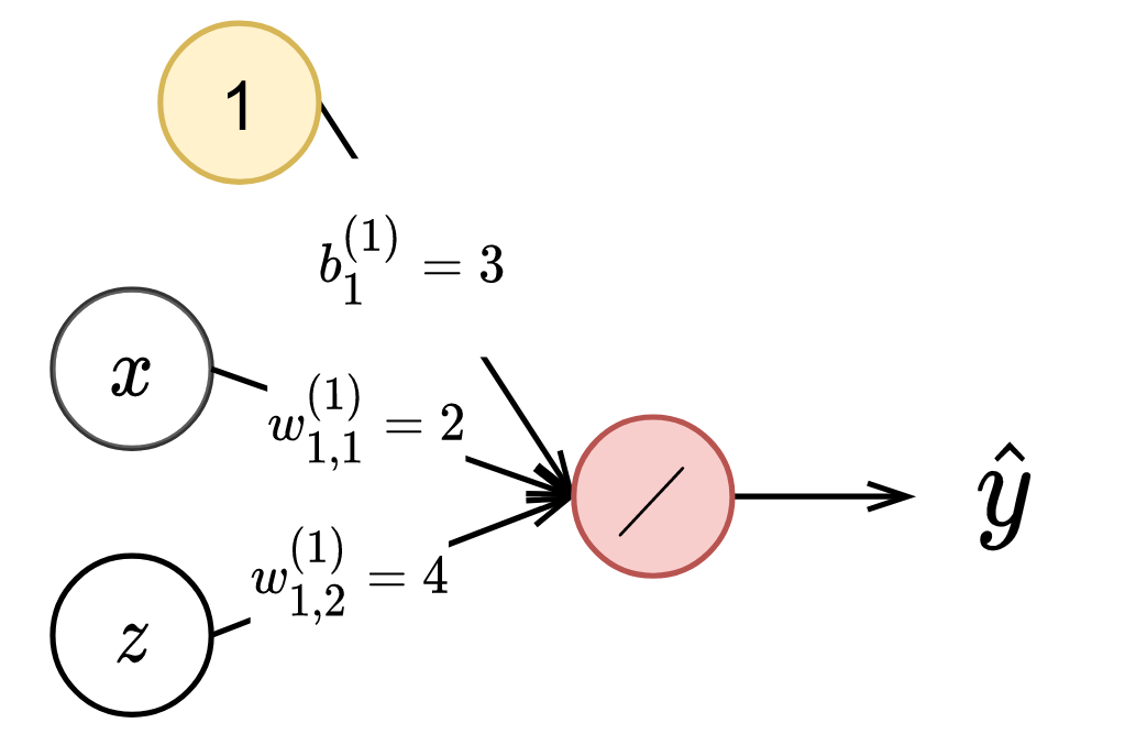
When an input is passed into a neural network, the input $x$ is multiplied by respective weights (denoted by $w$) and added to by a bias term $b$, resulting in a new value represented within a hidden node. In our model, we set the number of nodes in each layer to $n$. Each node, along with its incoming edges, represents some inner function. As our neural network can have many nodes and many layers, neural networks can be thought of as a composition of these inner functions to produce a more complex, outer function $f$ described above. The backslash in the most-right node represents a summation, resulting in a scalar value output. Now we will discuss precisely how to produce an output $\hat{y}$ given an input $x$ through learning a mapping.
Forward Propagation
The final output $\hat{y}$ is computed from the node values and weights of the previous layer, in our case, layer 2. We can multiply the output of the hidden nodes in layer 2, denoted by $o^{(2)}_i$, where $i$ represents a node index from $i$ to $n$ (i.e., $i \in \{1,2,\ldots,n\}$, by the weights connecting these nodes with the output node and add the bias term b^{(3)}_{i}. We display this process in Equation 1.
\begin{align}
\hat{y} = \sum_{i=1}^n w_{1,i}^{(3)} o^{(2)}_i + b^{(3)}_{1}
\end{align}
But, what is $o_i^{(2)}$ equal to? We display how $o_i^{(2)}$ is computed in Equation 2.
\begin{align}
o_i^{(2)} = g(z_i^{(2)})
\end{align}
Here, $i$ is again the node index and $g$ is an activation function (i.e., $g: Z \rightarrow O$). Neural networks cannot represent nonlinear functions without utilizing nonlinear activation functions. Activation functions help neural networks represent more complex functions by transforming node values by a nonlinear function. Common activation functions used include ReLU, tanh, sigmoid, etc. Here, we will discuss and use the ReLU (Rectified Linear Unit) as our activation function.
For our example, we will use the ReLU activation function, as shown in Equation 3.
\begin{equation}g(z) =\bigg\{\begin{aligned} &z \text{ if }z \geq 0\\ &0 \text{ otherwise}\end{aligned}\bigg\}\end{equation}
It is also helpful to know the gradient of the ReLU function, displayed in Equation 4.
\begin{equation}g'(z) =\bigg\{\begin{aligned} &1 \text{ if }z \geq 0\\ &0 \text{ otherwise}\end{aligned}\bigg\}\end{equation}
Moving back to Equation 2, we solve for $z_i^{(2)}$ in Equation 5.
\begin{align}
z^{(2)}_i = \sum_{j=1}^n w_{i,j}^{(2)} o^{(1)}_j + b^{(2)}_{i}
\end{align}
This procedure can be used throughout the neural network, computing the current layer using the previous layer’s output. For simplicity of algorithmic notation, you can consider the neural network’s input, $x$, as $o^{(0)}$. Here, $o^{(0)}$ represents the hypothetical output of a hypothetical zeroth layer. In Algorithm 1, we display the complete forward propagation algorithm, expressing the layer number as a variable for generalizability. This algorithm computes a predicted output, represented by $\hat{y}$, given input features, $x$.
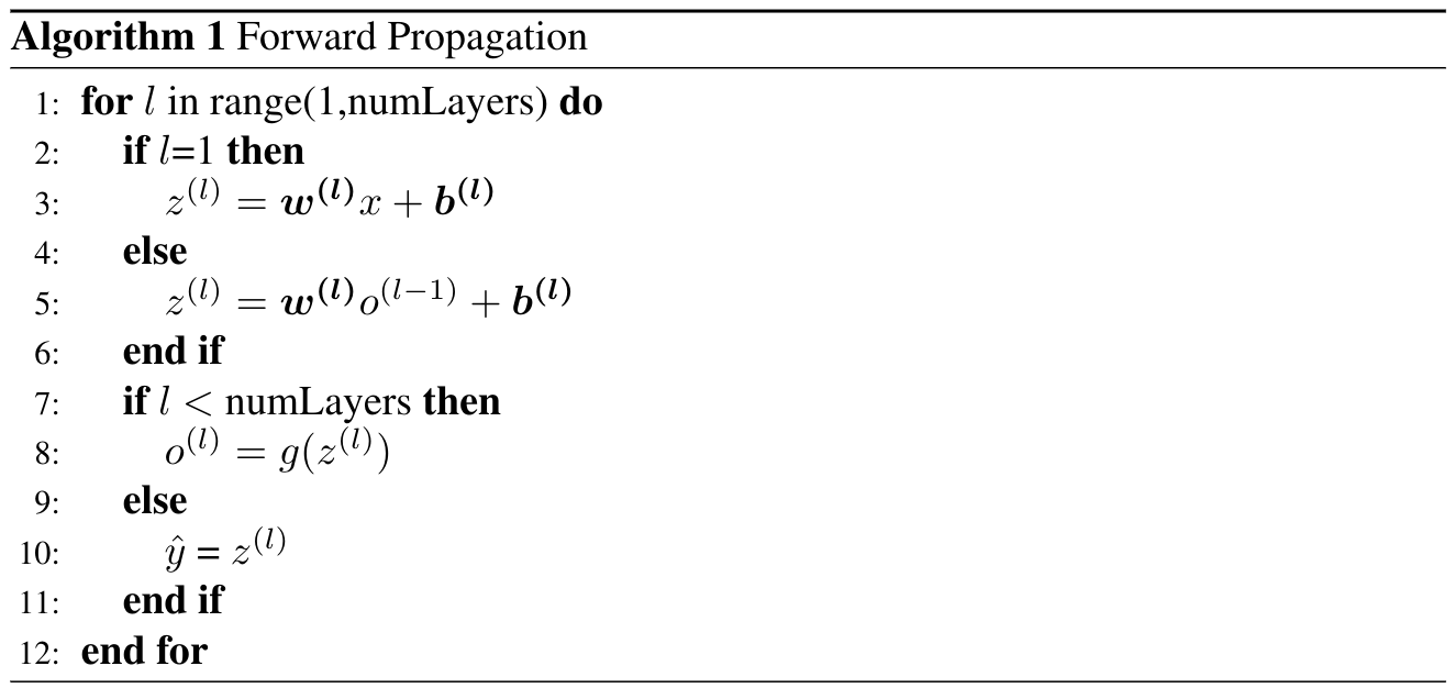
We can now analyze the computational complexity of this algorithm. For the sake of simplifying the analysis, we assume the number of layers in the neural network, $l$, is equal to the number of nodes in each layer, $n$, which we also set as equal to the size of the input, $|x|=d$. Thus, $n=l=w$. In Algorithm 1, Steps 3 and 5 represent a matrix multiplication combined with addition. This process has a complexity of $O(n^2+n)$. As a reminder, for any matrix multiplication of two matrices of size $p \times q$ and $q \times r$, respectively, the computational complexity of this multiplication is $O(pqr)$. Thus, since we are multiplying weight matrices of size $n \times n$ to a vector of size $n \times 1$, the complexity of the matrix multiplication alone is $O(n \times n \times 1) = O(n^2)$. The addition operation adds complexity $O(n)$, resulting in $O(n^2+n)$ for Steps 2-6. Steps 8-10 have a complexity of $O(n)$ leading, resulting now in the complexity $O(n^2 + 2n)$. Since Step 1 iterates $n=l$ times, we arrive at a total complexity of $O(n(n^2 + 2n))=O(n^3)$ for Algorithm 1.
Now that we can perform a forward pass and know its complexity, we can discuss how to update our weights and attempt to learn a model that fits the data.
Backpropagation
To optimize our neural network weights to more accurately represent our data, we first establish a loss function that quantifies our model’s error (i.e., how wrong its outputs are for a desired task). Given this loss function, we could then compute the gradients of our loss function with respect to each weight. We could then perform gradient descent to optimize our model parameters as we did in the gradient descent blog post. However, we will now do something a bit more sophisticated to make the optimization process more computationally efficient.
Let’s consider a common loss function, as shown in Equation 6. This loss function represents a mean-squared error loss between the true label (true y-value in the data) and the predicted value using our neural network ($\hat{y}$).
\begin{align}
L=\frac{1}{2} (y-\hat{y})^2 = \frac{1}{2} (y-f(x))^2
\end{align}
The derivative of this loss function with respect to $w_{1,1}^{(1)}$ is displayed in Equation 7 according to chain rule.
\begin{align}
\frac{\partial L}{\partial w_{1,1}^{(1)}} = (y-\hat{y}) * \frac{\partial \hat{y}}{\partial w_{1,1}^{(1)}} \bigg|_x
\end{align}
So, how do we comput $\frac{\partial \hat{y}}{\partial w_{1,1}^{(1)}}$? There are 4 paths from the output node to $w_{1,1}^{(1)}$, which highlighted in blue in Figure 4. The upper-most path has the gradient shown in Equation 8.
\begin{align}
\frac{\partial \hat{y}}{\partial w_{1,1}^{(1)}} = \frac{\partial \hat{y}}{\partial o^{(3)}} \frac{\partial o^{(3)}}{\partial z^{(3)}} \frac{\partial z^{(3)}}{\partial o^{(2)}_1} \frac{\partial o^{(2)}_1}{\partial z^{(2)}_1} \frac{\partial z^{(2)}_1}{\partial o^{(1)}_1} \frac{\partial o^{(1)}_1}{\partial w_{1,1}^{(1)}}
\end{align}
The rule for computing the “total derivative” encompassing all of these paths can be seen through an example here.
Computing a single partial derivative is computationally expensive, and computing each weight’s partial derivative individually (e.g., (e.g., $\frac{\partial \hat{y}}{\partial w_{1,1}^{(1)}}$ and then $\frac{\partial \hat{y}}{\partial w_{1,2}^{(1)}}$) and so forth all the way to $\frac{\partial \hat{y}}{\partial w_{1,n}^{(l)}}$) would be terribly inneficient.
If we instead look at $\frac{\partial \hat{y}}{\partial w_{1,2}^{(1)}}$, you can see that it shares many of the same nodes as $\frac{\partial \hat{y}}{\partial w_{1,1}^{(1)}}$. In Figure 5, we display a depiction of gradient computations required for $w_{1,1}^{(1)}$, $w_{2,1}^{(1)}$, and the overlap in the computations.

We would like to take advantage of this overlap in computation, which is exactly where the Backpropagation algorithm comes in. Backpropagation is a form of reverse-mode automatic differentiation that allows us to eliminate redundant computation in applying the chain rule to compute the gradient of our neural network.
Applied to neural networks, the backpropagation algorithm starts from the last layer of the neural network, computes an error term (denoted as $\delta$), and multiplies this error term by the gradient. The algorithm computes each node’s respective gradient in memory and reuses these variables as the algorithm continues, backpropagating the information for efficiency. We display the algorithm for Backpropagation in Algorithm 2. The output of the Backpropagation algorithm is gradients for each set of weights and biases.
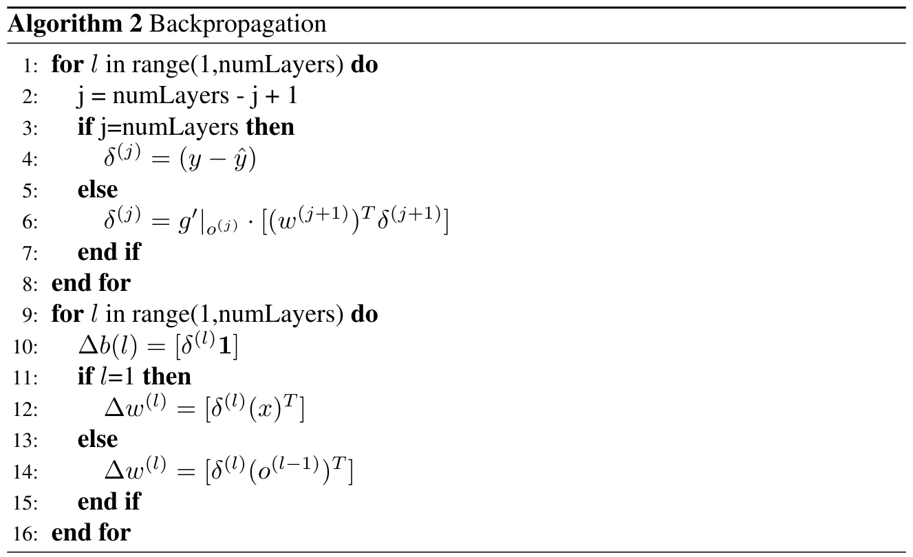
Looking at the computational complexity of this algorithm, we see Step 4 has a complexity of $O(1)$. Step 6 has a complexity of $O(n^2 + n)$ or $O(n^2)$. Step 10 has a complexity of $O(n)$. Steps 12 and 14 both have complexities of $O(n^2)$. Since we iterate over the number of layers, equal to $n$ for our analysis, the total complexity is $O(n^3)$. If we did not use the Backpropagation algorithm, we would end up redundantly computing each component’s derivatives multiple times. Using the previous assumptions setting the cardinality of $|x|$, the number of nodes, and the number of layers to $n$, we would be iterating over $O(n^3 + n^2)$ weight derivatives resulting in a total complexity of $O(n^6)$.
The last step in optimizing our neural network model to minimize our loss function is to update weights and biases. Equations 9-10 show one step of gradient descent using the derivatives from our backpropagation procedure in Algorithm 2. Note that Equations 9-10 represent only one step of gradient descent, so one would need to iteratively perform the forward pass, then backward pass, then parameter updates (Equations 9-10) until the model converges to a local minimum, as described in our previous post on gradient descent.
\begin{align}
w^{(l)} \to w^{(l)} + \alpha \Delta w^{(l)}
\end{align}
\begin{align}
b^{(l)} \to b^{(l)} + \alpha \Delta b^{(l)}
\end{align}
We now have the ability to train neural networks in a computationally efficient manner, which, in turn, allows us to do more training iterations per unit time, which should help us train more accurate neural networks!
Key Points throughout this Blog:
- Neural networks can be used to represent almost any function.
- Forward propagation is the process of taking input features, $x$, and computing an output in the form of a model’s estimate, $\hat{y}$.
- We can use the difference in the output, $\hat{y}$, of the neural network and our ground-truth data, $y$, to compute a loss, and then use this loss value to compute gradients in the backpropagation algorithm.
- Backpropagation is a special case of reverse-mode automatic differentiation and allows for efficient gradient computation. The result is that the training of extremely large neural networks is possible!
