Value iteration and Q-learning make up two fundamental algorithms of Reinforcement Learning (RL). Many of the amazing feats in RL over the past decade, such as Deep Q-Learning for Atari, or AlphaGo, were rooted in these foundations. In this blog, we will cover the underlying model RL uses to describe the world, i.e. a Markov decision process (MDP), as well as two algorithms for performing RL: value iteration and Q-learning. By the end of this blog post, you should be able to understand the connection between value iteration and Q-learning and how to employ either of these algorithms to learn the optimal policy.
This post is divided into three parts:
- Markov decision processes
- Value functions and Value iteration
- Q-learning and Deep Q-learning
Prerequisites:
The only prerequisites you will need to understand this blog are gradient descent and backpropagation. Both of these topics were covered in our first two blogposts (week 1 and week 2).
Markov Decision Processes
An MDP is a 5-tuple describing an environment consisting of the following five components:
- States: A state, $s$ is any predefined momentary instance in the world that an agent can exist in. For the rest of this post, we will use the variable $S$ to represent the set of all possible states in the world with $s \in S$ referring to an individual state.
- Actions: An action, $a$, is an event facilitated by the agent that can transition you from one state to another provided that such a transition is possible MDP. We will use $A$ to represent the set of all possible actions in the world, with $a \in A$ referring to an individual action. We note that actions may not have deterministic consequences. For example, flipping a coin may not give you the same result each time! The degree to which actions have deterministic effects is described by the transition function.
- Transition function: The transition function is a function that defines the probability of moving to a specific next state, given your current state and a valid action. The transition function, $T$, is mathematically defined as follows, $ T: S \times A \times S’ \rightarrow [0,1]$.
- Reward: The reward function specifies a real number value that defines the efficacy or a measure of “goodness” for being in a state, taking an action and landing in the next state. Similarly to the transition function, the reward is defined as follows, $R: S \times A \times S’ \rightarrow \rm I\!R $. Note that the state you end up in may be uncontrollable since state transitions can be dynamic.
- Discount Factor: The discount factor can be specified using $\gamma$, where $\gamma \in [0,1)$. Note the non-inclusive upper bound for the discount factor (i.e., $\gamma \neq 1$). Disallowing $\gamma = 1$ allows for an MDP to be more mathematically robust. Specifically, the goal for RL algorithms is often to maximize discounted reward across time. Consider the case of an infinite horizon MDP (i.e., the MDP never ends) in which the rewards are always positive. If the discount factor, $\gamma$, is equal to 1, then the sum of future discounted rewards will be infinite, making it difficult RL algorithms to converge (i.e., know when they can stop determine which actions should be taken in each state). Thus, the choice of gamma is a critical for the success of RL algorithms, e.g. Q-learning and value iteration.
You may have read about a concept known as Markov chains. While Markov Chains will not be covered in this post, it is important to understand the distinction between markov chains and markov decision processes, as both concepts share the markov property. Fundamentally, a markov chain consists of the components of a markov decision process except actions, rewards, and a discount factor. An agent in a markov chain is not in control of their movements, the world is in control of the agent’s movements. In a markov decision process the agent has an influence on the outcomes. Thus the transition function of a markov chain is simply defined as $T: S \times S’ \rightarrow [0,1]$.
Markov Property: The markov property holds when the next state depends only on the current state and current action and is independent of the history of states and actions prior to that.
Nota bene: In some MDPs, you may see the initial state distribution included as a part of the MDP. While that is still a valid representation, in this blog, we are going to remain agnostic of the initial state distribution.
Value functions and Value Iteration
The value function, $V(s)$, is a measure of the expected reward you can receive from any given state $s$ given an MDP and a policy describing which actions an agent takes in each state. Formally, a policy, $\pi: S \rightarrow [0,1]^{|A|}$, is a probability distribution over actions, $a \in A$, conditioned on a state, $s$. For the sake of this blog, we will consider a policy to be deterministic (i.e., $\pi(s,a) = 1$ for a single action, $a$, and $\pi(s,a’)=0$ for all other $a’ \neq a$). Having defined a policy, we can now mathematically define the value function for a policy: $$V^{\pi}(s) = E[\sum_{t=0}^{\infty} \gamma^t r_t | \pi, s_0 = s]$$ In a deterministic world, this expectation could be ignored; however, in general, we include the expectation as both the policy (e.g., an agent that doesn’t always like the same thing for breakfast) and the transition function (e.g., how bad traffic is) could describe nondeterministic attributes of the problem we want to model.
The goal of Value Iteration is to find a policy that maximizes the value function: $$\pi^*(s) = argmax_{\pi \in \Pi} V^{\pi}(s), \forall s \in S $$ In this equation $\Pi$ represents the set of all possible policies within the MDP, and $\pi^*(s)$ is the optimal policy. What the value function equation (i.e., $V^{\pi}(s) = E[\sum_{t=0}^{\infty} \gamma^t r_t | \pi, s_0 = s]$) states is that you are going to follow a policy, $\pi$, starting at state, $s$, for up to an infinite number of time steps, $t$, proceeding forward from $t=0$ to $t = \infty$ along a trajectory (i.e., a sequence of state-action pairs, $(\langle s_1,a_1 \rangle , \langle s_2,a_2 \rangle,\ldots)$), where the accumulated reward, $r_t$, is discounted via multiplication with $\gamma^t$. This process of discounting rewards means that, the further you go into the future, rewards have a diminishing impact on value or “goodness” of being in state, $s$. Adjusting $\gamma$ allows you to define your preferences towards optimizing for short-term vs long-term gain. The expectation matters because, as stated in the previous paragraph, transitions can be non-deterministic, thus the expectation provides a normalized estimate of the discounted reward.
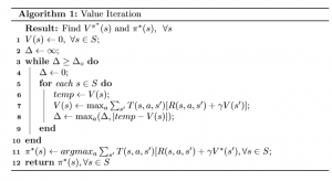
Value iteration is a computational algorithm that provides a means of finding the optimal policy, $\pi^*$. The algorithm works by iteratively determining the value of being in each state, $s,$ assuming that the agent takes the best possible action in that state under the current estimate of the value function. The value iteration algorithm is shown in the figure below.

This algorithm iteratively updates the value, $V(s)$, for each state, $s$ until it reaches a point where the change in value is negligible, as defined by the threshold $\Delta_\circ$. Take note of Line 7 in this algorithm in which we consider a state, $s$, an action, $a$, and the resulting state, $s’$, in a sequence, $\langle s, a, s’ \rangle$. Line 7 works by updating the value for the given state, and is called the value update and is reminiscent of Bellman’s optimality condition. This condition says $$ V(s) = \max_{a \in A} E [R(s,a,s’) + \gamma \max_{a’}V(s’)] = \max_{a \in A} \sum_{s’\in S} T(s,a,s’)[R(s,a,s’) + \gamma V(s’)]$$
When this condition holds for a given state, $s$, we would find in Line 8 that $temp – V(s) = 0$. If the condition holds for all states, $s$, then the value function has converged to the optimal value function, $V^{*} = V^{\pi^*}$, and the optimal policy, $\pi^*$, can simply be exctracted by Line 11. In a sense, Value iteration works by iteratively pretending or enforcing (Line 7) that Bellman’s optimality condition holds, measuring if the condition does not hold (Line 8), and, terminating once the condition holds within an acceptable margin of error (Line 3).
Upon convergence (i.e., reaching an acceptable level of error, $\Delta < \Delta_0$), this Value Iteration returns a value function, $V^{*}$, that provides an estimate of the future expected reward while following the optimal policy, $\pi^*$, as well as the optimal policy itself. To be perfectly clear, we should note that the actual value function and policy returned are only approximately optimal, and it would be more technically accurate to refer to them as $V \approx V^*$ and $\pi \approx \pi^*$.
Nota Bene: In some textbooks the bellman’s update equation may be alternatively defined, considering the reward function to be independent of the next state $s’$, i.e. $$V(s) \leftarrow \max_a R(s,a) + \sum_{s’} T(s,a,s’)\gamma V(s’)$$ However the update rule shown in the value iteration algorithm above is a more complete representation of the value estimate because you cannot always assume that, for any given MDP, your reward will not depend on the next state.
Let us now define surrogate terms, the Q-value and the Q-function. Similar to the value function, the Q-function is a quality measure. However the unlike the value function, the Q-function measures the expected discounted reward for taking a particular action at a given state, i.e. $R: S \times A \rightarrow \rm I\!R$. We refer to the Q-value as what the Q-function returns.
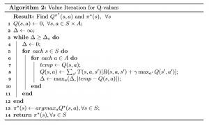
Although Q-learning is the go-to algorithm for estimating Q-values and consequently optimal policies from these Q-values, you may also modify the value iteration algorithm to solve for the Q-values.

There are two primary differences between both algorithms resulting from an introduction of a Q-function. First, since the Q-function is dependent on both states and actions, we need to loop through all possible actions (Line 6) as well as the set of all states. Second, you’ll notice that the update rule (Line 8) has changed upon incorporating the Q-function. Since the estimate for the optimal Q-value, $Q(s’,a’)$, for the next state, $s’$, depends on the next action, $a’$, we need to replace “$V(s’)$” from Line 7 of Algorithm 1 with “$\max_{a’} Q(s’,a’)$” in Line 8 of Algorithm 2.
We note that Algorithms 1 and 2 are often referred to as flavors of “exact RL” because, unlike in function approximation algorithms commonly used in RL (i.e., deep learning-based RL), here, we are guaranteed to able to solve for the true, optimal Q-values within a margin of error, $\Delta$, and given sufficient computational resources. “Approximate” RL techniques (e.g., deep RL) do not typically have such guarantees.
An important question to answer is, then, “Why do we not do this in practice instead of Q-learning?” Unfortunately, most real-world applications of RL contain too many states to iterate over even once, let alone the multitude of times required for the algorithm to converge to an acceptable error threshold. Hence, function approximation algorithms, such as Deep Q-learning are preferred.
Q-Learning and Deep Q-learning
Prior to discussing Q-learning itself, let us define a term called the Bellman Residual.
$ \delta(s,a,s’) = [R(s,a,s’) + \gamma \max_{a’}Q(s’,a’)] – [Q(s,a)] $$
The bellman residual, denoted by $\delta$, computes a measurement error for Q-learning to describe how wrong the current estimate of the Q-function is given a transition sequence, $\langle s,a,s’ \rangle$. When the Q-function is optimal, we should find that the modified form of the Bellman optimal condition holds: $$Q(s,a) = E[R(s,a,s’) + \gamma \max_{a’\in A} Q(s’,a’)] = \sum_{s’} T(s,a,s’)[R(s,a,s’) + \gamma \max_{a’\in A} Q(s’,a’)]$$
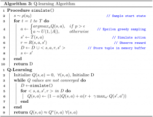
When this condition holds, we should find that $ \delta(s,a,s’) = 0 $ for all possible transition sequences. However, when we first initialize a Q-function, as we do in Line 2 of Algorithm 3, our Q-function will almost certainly be wrong, and $ \delta(s,a,s’)$ will not equal zero. So, how do we improve our Q-function to be correct?
The way Q-learning works is by “blending” our current estimate of the Q-function, $Q(s,a)$, with a “point-estimate” of what the Q-function should be, i.e. $R(s,a,s’) + \gamma \max_{a’}Q(s’,a’)$. The degree of blending is controlled by a hyperparemeter, $\alpha$ in the following equation: $$ Q(s,a) = (1 – \alpha) Q(s,a) + \alpha (R(s,a,s’) + \gamma \max_{a’}Q(s’,a’)) $$
If $\alpha = 1$, then we completely ignore our current estimate of the Q-function. If $\alpha=0$, then we completely ignore new information. A decent starting place for setting $\alpha$ in practice is to choose $\alpha = 0.99$, which puts most of the emphasis on the current estimate of the Q-function. However, we encouage you to experiment with this parameter!
The full algorithm for Q-learning is shown in the algorithm pictured below.

It is important to note that, unlike in the version of the bellman equation described earlier, Q-learning does not include a transition function in its Bellman update equation! In Q-learning, we instead simulate actions within the environment and utilize the states visited during the simulation (i.e., the trajectory) to apply the bellman equation. The simulate function in the algorithm shows how trajectories are sampled in Q-learning. In each timestep of the trajectory, we use an epsilon-greedy sampling strategy to select an action. If a randomly sampled probability is greater than a predefined $\epsilon$ value, then we greedily sample the action, otherwise we randomly sample an action from the space of all actions. Upon selection, we simulate that action and observe the next state and reward received for that action. Finally we store all this observed information into the memory buffer, update the current state and repeat this process until we reach a terminal state. The trajectory computed from each simulation is then used to update the Q-values via the Bellman update equation (line 6 in Q-learning).
The absence of a transition function makes Q-learning a model-free RL algorithm, as it does not need any prior knowledge of “the world” to learn the optimal policy. This model-free characteristic is significant because, in practice, you rarely have access to the transition probabilities for all state action pairs in real-world application.
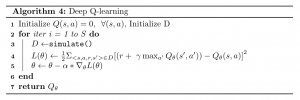
With enough time and sampled trajectories, Q-learning will be able to estimate the optimal Q values for each state action pair. However, as currently constructed, the Q-learning algorithm requires a lookup table for each possible state action pair, and filling in those values. The size of the state-action spaces in real-world tasks makes maintaining a lookup table of Q-values infeasible. One possible solution to this lack of computational power is the use of function approximation techniques, e.g. Deep Q-learning. The term “deep” comes from parameterizing Q-values using neural networks. Therefore, instead of learning a literal table of Q-values, our goal shifts towards learning the weights of a neural network that can output the Q-value for any given state action pair. Employing the square of the Bellman residual as our loss function, we can apply the backpropagation algorithm (Covered in Week 2) to learn the weights of the Q-network.

When compared to Q-learning, there are three primary reasons why Deep Q-learning is better suited for real world applications,
- Not enough memory: Q-learning requires storing a lookup table of all states and actions, leading to an infeasible RAM requirement for most modern applications.
- Not enough time: Deep Q-learning is often significantly faster to train because of the ability to incorporate techniques like batched gradient descent and adaptive optimization. In addition to this, Deep Q-learning does not require convergence of the Q-value for each state action pair.
- Interpolation: Deep Q-Learning is a function approximation algorithm. Because the Q-network approximates Q-values for states and actions, we can assume that the network can interpolate q-values for similar state and action pairs i.e, $ Q(s,a) \approx Q(s’,a’)$ if $(s,a) \approx (s’,a’)$. In practice, Deep Q-learning is more efficient than seeking convergence for each individual state-action pair. However, there are pathological cases where this may not be true, for example, when the slightest change in the state or action may result in drastically different outcomes.
While we have not yet covered enough yet to fully implement Deep Q-learning and understand the tips-and-trick in practically implementing a Deep Q-learning model, please stay tuned for a future blog on that topic!
Key Takeaways from this blog:
- A Markov Decision Process(MDP) is a tuple used to describe an environment and is made up of components used in reinforcement learning algorithms.
- The goal of most reinforcement learning algorithms is to maximize the cumulative expected reward, which is also known as the value function.
- Value iteration is an iterative algorithm that uses the bellman equation to compute the optimal MDP policy and its value.
- Q-learning, and its deep-learning substitute, is a model-free RL algorithm that learns the optimal MDP policy using Q-values which estimate the “value” of taking an action at a given state.
