Gradient descent is an ubiquitous optimization algorithm used to train machine learning (ML) algorithms from simple linear regression models to sophisticated transformer architectures. ML researchers are typically introduced to unconstrained optimization problems (e.g., least-squares, LASSO, or Ridge regression). However, many really-world ML problems are constrained optimization problems. For example, in robotics, we may want to train a robot for maneuvering around a crowd by imitating human motion (e.g., Behavior Cloning where the robot minimizes the divergence between the distribution of actions the robot takes and that the human would take in the same state of the world, $x$) subject to the constraint that the robot will never crash into a person.
In this blog post, we will look at some powerful approaches for performing constrained optimization. First, we quickly recap the concept of gradient descent. Next, we’ll delve into Projected Gradient Descent, a technique that introduces constraints to the optimization process. Finally, we’ll uncover the magical world of Mirror Gradient Descent, a method that combines the power of duality and optimization. For an example of how Mirror Gradient Descent has been used, check out these papers:
- Montgomery, W.H. and Levine, S., 2016. Guided policy search via approximate mirror descent. Advances in Neural Information Processing Systems, 29.
- Zhang, M., Geng, X., Bruce, J., Caluwaerts, K., Vespignani, M., SunSpiral, V., Abbeel, P. and Levine, S., 2017, May. Deep reinforcement learning for tensegrity robot locomotion. In 2017 IEEE international conference on robotics and automation (ICRA) (pp. 634-641). IEEE.
- Cheng, C.A., Yan, X., Wagener, N. and Boots, B., 2018. Fast policy learning through imitation and reinforcement. arXiv preprint arXiv:1805.10413.
Recap: Gradient descent
Imagine we are trying to train a neural network with a parameter \(\theta\). Given \(\theta\), the neural network produces the prediction \(f(\theta)\). We have a cost function \(\mathcal{L}(\theta)\). Our goal is to find the optimal parameter $\theta^*$ that minimizes \(\mathcal{L}(\theta)\). Let’s consider the standard \(L^2\)-norm loss function with respect to our dataset \(D\), defined as follows:
\[\mathcal{L}(\theta) = \Sigma_{(x,y) \in D} \frac{1}{2} ||y-f_\theta (x)||^2 .\]
Starting from an initial point \(\theta_0\), Gradient Descent performs the following update at every timestep:
\[\theta_{t+1} \leftarrow \theta_t -\alpha \nabla_\theta \mathcal{L}(\theta_t).\]
Note that we are going opposite to the gradient direction (minus sign in the gradient) since we are “minimizing” the loss function. When the dataset is too large to compute the gradient at every timestep, we use Stochastic Gradient Descent which computes the gradient with respect to a single example, or Mini-batch Gradient Descent which computes the gradient with respect to a small batch sampled from the dataset at every timestep.
For more information such as time complexity and convergence rate, please refer to our previous blog post: Bootcamp Summer 2020 Week 1 – Gradient Descent.
Constrained Optimization Problem
In many real-world scenarios, optimization problems are often attached to certain constraints or boundaries that resulting parameters must satisfy. These constraints can represent physical limitations, practical considerations, or desired properties of the solutions. For example, consider a manufacturing company that produces various products. The company aims to maximize the overall utility derived from these products, taking into account factors such as customer demand, quality, and profitability. However, the company faces a budget constraint, which limits the total amount of money available for production.
To formulate this as a constrained optimization problem, let’s first define the following variables:
$x_1, \cdots, x_n$: The quantities of each product to be manufactured.
$U(x_1, \cdots, x_n)$: The utility function that quantifies the overall satisfaction derived from the products.
$c_1, \cdots, c_n$: The respective costs of producing each product.
The objective is to maximize $U(x_1, x_2, \cdots, x_n)$ while satisfying the constraint of the total budget, $B$. Mathematically, the constrained optimization problem can be formulated as:
\begin{align*}
Maximize_{x_1, \cdots, x_n} \text{ } & U(x_1, \cdots, x_n)\notag\\
\text{subject to } & \Sigma_{i=1}^n x_i*c_i \leq B.\notag
\end{align*}
This example highlights the need for algorithms to solve such constrained optimization problems that arise in various fields, such as resource allocation, portfolio optimization, and image reconstruction.
Projected Gradient Descent
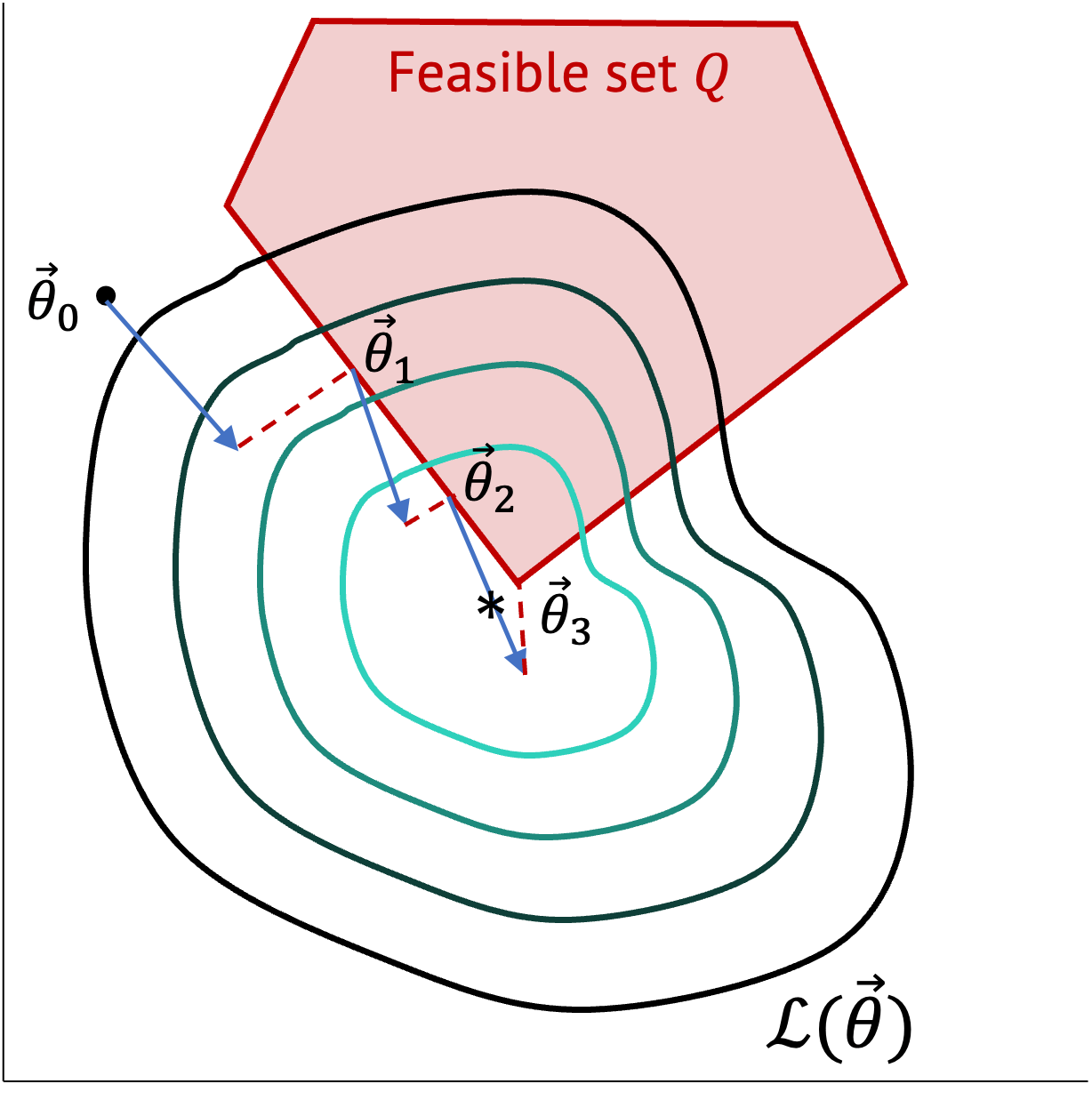
Then, how can we incorporate the constraints into the optimization process so that we can balance between optimizing the objective function and constraining parameters? Projected Gradient Descent (PGD) addresses this challenge by ensuring that the iteratively updated parameters belong to the feasible region defined by the constraints.
The key idea behind PGD is to project the current solution onto the feasible region at each iteration. This projection step involves mapping the updated parameter onto the closest point within the feasible region in case if lands outside of it, effectively “projecting” it onto the constraint boundaries. By doing so, PGD guarantees that the resulting parameters remain feasible throughout the optimization process.
To illustrate, let’s consider a constraint \(A\theta = b\) for our optimization problem. Assume Q is the feasible set for the constraint (the red region from Fig. 1) and P is the projection function onto $Q$:
\[Q = \{\theta|A\theta = b\},\]
\[P: \theta’ \mapsto arg\,min_{\theta \in Q} \frac{1}{2} ||\theta – \theta’||^2 .\]
Projected gradient descent is defined as follows:
\[\theta_{t+1} \leftarrow P(\theta_t – \alpha_t \nabla_\theta \mathcal{L}(\theta_t)).\]

For the Lipshitz constant \(L\) and the step-size \(\alpha_t = \frac{R/G}{\sqrt{t}}\), it is known that if \(R \geq ||\theta_0 – \theta||_2\) and the gradient of \(\mathcal{L}\) is bounded by a constraint \(G\), i.e., \(G \geq ||g||_2\), \(\forall g \in \frac{\partial \mathcal{L}}{\partial \theta}\), the inequality \(\mathcal{L}(\theta_t) – \mathcal{L}(\theta^*) \leq C \frac{L}{\sqrt{t}}\) holds.
Mirror Gradient Descent
Mirror Gradient Descent (MGD) is a fascinating optimization technique that combines the power of optimization with the concept of duality. It draws inspiration from convex duality, a fundamental concept in convex optimization that establishes a relationship between primal and dual problems. MGD exploits this duality to transform the original optimization problem into a dual problem and solves it using a gradient descent-like approach.
In MGD, the optimization process involves iteratively updating the primal parameter in the primal space, while simultaneously updating the corresponding dual parameter in the dual space. The updates are performed by taking steps in the direction opposite to the gradients of the primal and dual objectives. This dual update is analogous to a mirror reflection of the primal update, which is the reason why this algorithm is called by the name “Mirror Gradient Descent.”
The motivation to work in the dual space is that it can often be simpler or have desirable geometric or algebraic properties, leading to more efficient optimization. MGD has been applied to various domains, including convex optimization, machine learning, and signal processing. It offers a powerful framework to tackle optimization problems with complex constraints or objectives, leveraging the interplay between primal and dual updates to achieve efficient convergence and desirable parameters.
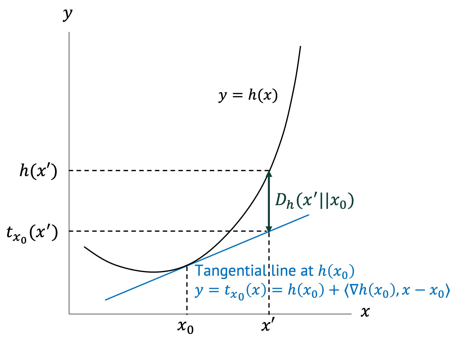
Before we dig into MGD more, let’s first define Bregman Divergence of a function \(h\) as \(D_h (x’||x)\).
\[D_h (x’||x):= h(x’)-h(x)-\langle \nabla h(x), x’-x \rangle \]
(\(\langle \cdot,\cdot \rangle\) is dot product.)
If we do the first order Taylor expansion of a function $h$, the tangential line at \(h(x)\) crosses a point \((x’, h(x) + \langle \nabla h(x), x’-x) \rangle) \). Bregman Divergence \(D_h (x’||x)\) is the gap between \(h(x’)\) and \(h(x) + \langle \nabla h(x), x’-x) \rangle \). It becomes large when the function \(h\) is steeper.

Mirror gradient descent is defined as follows:
\[\theta_{k+1} \leftarrow arg\,min_\theta {\langle \alpha_k \mathcal{L}(\theta_k), (\theta – \theta_k) \rangle + D_h (\theta||\theta_k)}. \]
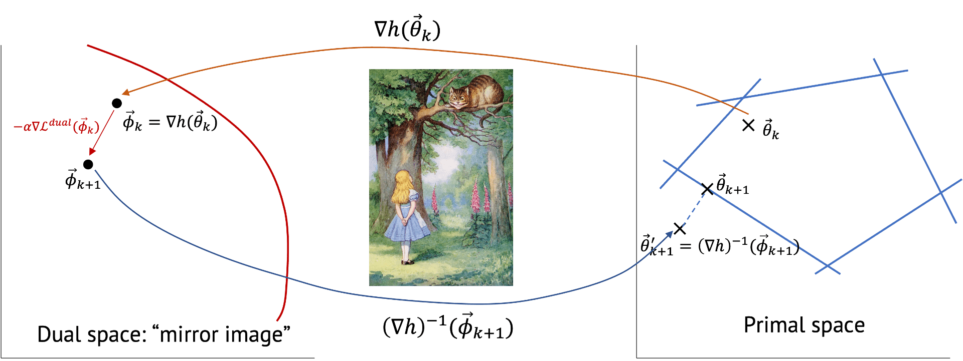
The concept of mirror gradient descent is that we first transform (with \(\nabla h(\theta_k)\)) the primal space of \(\theta\) into the dual space of \(\phi\) which possibly have an easier geometry, update the parameter, and do inverse-transform to come back to the primal space.

Now, let’s first get a mirror image in the dual space and then project it back (with \((\nabla h)^{-1} (\phi_{k+1}))\) to the primal space.
\begin{align*}
0 & = \frac{\partial}{\partial \theta} \{\alpha \langle \nabla \mathcal{L}(\theta_k), \theta_{k+1}-\theta_k \rangle + h(\theta_{k+1}) – h(\theta_k) – \langle \nabla h(\theta_k), \theta_{k+1} – \theta_k \rangle \} \\
& = \alpha \nabla \mathcal{L}(\theta_k) + \nabla h(\theta_{k+1}) – \nabla h(\theta_k)
\end{align*}
Finally, we get the update equation for mirror gradient descent:
\[\nabla h(\theta_{k+1}) = \nabla h(\theta_k) – \alpha \nabla \mathcal{L}(\theta_k) \]
\[ \theta_{k+1} \leftarrow (\nabla h)^{-1} [\nabla h(\theta_k) – \alpha \nabla \mathcal{L}(\theta_k)]. \]
Note that for constrained optimization program, the projection onto the feasible set can be applied afterward.
Example 1. For \(h(\theta)=\frac{1}{2}||\theta||^2\), Bregman Divergence becomes \(D_h(\theta||\theta_k) = \frac{1}{2} ||\theta-\theta_k||^2 \). Substituting Bregman Divergence and rewriting the update equation, we get
\[\theta_{k+1} \leftarrow arg\,min_\theta \{ \langle \alpha_k \nabla_\theta \mathcal{L}(\theta_k), (\theta – \theta_k)\rangle + \frac{1}{2} ||\theta – \theta_k||^2 \}.\]
Then,
\begin{align*}
0 & = \nabla_\theta f = \frac{\partial f}{ \partial \theta} \\
& = \frac{\partial}{\partial \theta} \{\langle \alpha_k \nabla_\theta \mathcal{L}(\theta_k), (\theta – \theta_k) \rangle + \frac{1}{2} ||\theta – \theta_k||^2\} \\
& = \frac{\partial}{\partial \theta} \langle \alpha_k \nabla_\theta \mathcal{L}(\theta_k), \theta \rangle – \frac{\partial}{\partial \theta} \langle \alpha_k \nabla_\theta \mathcal{L}(\theta_k), \theta_k \rangle + (\theta-\theta_k) \\
& = \alpha_k \nabla_\theta \mathcal{L}(\theta_k) + (\theta-\theta_k)
\end{align*}
which corresponds to the basic gradient descent \(\theta_{k+1} = \theta_k – \alpha_k \nabla_\theta \mathcal{L}(\theta_k) \). Indeed, gradient descent is a special case of mirror gradient descent with this \(h\). Another intuition for recognizing it is that for \(h(\theta)=\frac{1}{2}||\theta||^2\), \(\nabla_\theta h = \theta, (\nabla_\theta h)^{-1} = \theta \), i.e., the transform is one-to-one mapping. Hence, we get \(\theta_{k+1} = \theta_k – \alpha \nabla \mathcal{L}(\theta_k) \).
Example 2. \(h(\theta) = \Sigma_i \{\theta_i \ln(\theta_i) – \theta_i\} \) where $\theta$ satisfies \(\Sigma_i \theta_i = 1\).
\[\nabla h = [\ln(\theta_1), …, \ln(\theta_n)]^T, (\nabla h)^{-1} = \exp (\theta) \]
\[\langle \nabla h(\theta), \theta’ – \theta \rangle = \Sigma_i \frac{\partial h}{\partial \theta_i} (\theta’_i – \theta_i) = \Sigma_i (\ln \theta_i) (\theta’_i – \theta_i)\]
\[\Rightarrow D_h (\theta’||\theta) = \Sigma_i \{\theta’_i \ln(\frac{\theta’_i}{\theta_i}) – \theta’_i +\theta_i\} = \Sigma_i \theta’_i \ln(\frac{\theta’_i}{\theta_i})\]
using $\Sigma_i \theta_i = \Sigma_i \theta’_i = 1$. Note that with this $h$, Bregman Divergence converges to KL Divergence.
The update equation for mirror gradient descent becomes
\[\theta^{i}_{k+1} \leftarrow \exp(\ln(\theta_k) – \alpha \nabla \mathcal{L}(\theta_k)) = \theta_k \exp(-\alpha \nabla \mathcal{L}(\theta_k))\]
Typically, it’s good to use mirror descent if you are able to pick a good \(h\) for that class of problems.
There are also many other variants of gradient descent. Each algorithm possesses unique strengths, you may try to find what suits the best for your own optimization problem. Understanding and utilizing these techniques expands our problem-solving capabilities across diverse fields. So, please feel free to embrace these algorithms and explore their potential in your own endeavors.
Conclusion
Projected and Mirror Gradient Descent are powerful tools for constrained optimization problems in ML. These algorithms are more computationally expensive that regular gradient descent due to their need to address the constraints. The Bregman Divergence is an expressive way to represent many forms of optimization (e.g., Examples 1 and 2). Constrained optimization is key in safety-critical domains, such as ML for robotics and healthcare where constraint satisfaction must be enforced. Note: check out our blog post on KKT conditions for an alternative approach for constrained optimization: The method of Lagrange Multipliers.
Acknowledgements
This blog post was developed in part with support from course materials available at http://www.cs.cmu.edu/afs/cs.cmu.edu/academic/class/15850-f20/www/notes/lec19.pdf
