Gradient Descent (GD) is an intuitive optimization method. GD has become one of the most popular optimization methods in recent years due to its nice theoretical properties, effectiveness in real-world applications, and uncanny ability to train large-scale deep learning models. GD is commonly used in deep learning for finding neural network parameters that best capture patterns in the data. In this blog, we introduce three different flavors of GD, regular GD, Stochastic GD (SGD), and Minibatch GD (MbGD). We analyze these variants theoretically as well as empirically, and discuss which one is most appropriate for different scenarios! Finally, we discuss how GD can be improved or “accelerated” by adding “momentum”.
This blog is divided into four parts:
- Introduction of GD, SGD, and MbGD
- Analytical results
- Empirical results
- Accelerated GD
What is GD, SGD, and MbGD?
Let’s first look at a simple machine learning scenario. We have a dataset $\mathcal{D}=\{(x_i,y_i),\ i\in [n]\}$, where $(x_i,y_i)$ is “example” number $i$, $x_i$ is the input to a model we want to train and $y_i$ is the “label” we want our model to learn to predict from $x_i$. For instance, $x_i$ might be the date of the year, and $y_i$ might be the expected rainfall you would receive that day. In this simplified example, we assume $x_i$ is a scalar instead of a vector, but the concept and the math work for the vector case (where $x_i$ contains several features) too.
To allow us to visualize the model, let’s assume we are using a linear model parameterized by $\theta$ shown in Equation \ref{f}.
\begin{align}
f_\theta(x_i)=\theta x_i
\label{f}
\end{align}
The metric we use to judge our model (i.e., a “loss function”) is the Mean Squared Error (MSE) loss (Equation \ref{L}), which calculates the squared error for each prediction and averages over all data points.
\begin{align}
L(\theta)=-\frac{1}{2n}\sum_{i=1}^n(y_i-f_\theta(x_i))^2
\label{L}
\end{align}
We want to find the best model, $\theta^*$, according to our loss function (Equation \ref{loss}).
\begin{align}
\theta^*=\arg\min_\theta L(\theta)
\label{loss}
\end{align}
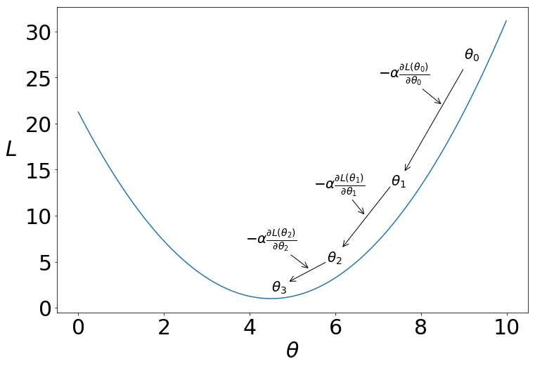
\(L\) is a quadratic function of the model parameter \(\theta\), illustrated in Figure 1. The problem then is to find the critical point, $\theta^*$, that is located at the minimum of this curve. To find the critical point, we set the first derivative of $L$ equals to $0$, i.e. $\frac{\partial L(\theta)}{\partial \theta}=0$. In the case of a simple linear model, we can directly solve for model parameters $\theta^*$. However, in deep learning, such direct methods do not exist. Instead, we need something else. In this tutorial, that “something else” is GD.

GD
In GD, we perform three steps:
- Calculate the gradient of our model parameters.
- Use the gradient to update model parameters.
- Repeat steps 1 and 2 until a pre-set tolerance is achieved.
We use $\nabla$ as the gradient operator and it is defined in Equation \ref{gradient}.
\begin{align}
\nabla_\theta=\left[\begin{matrix}
\frac{\partial}{\partial \theta_1}\\
\frac{\partial}{\partial \theta_2}\\
\cdots\\
\frac{\partial}{\partial \theta_m}\\
\end{matrix}\right]
\label{gradient}
\end{align}
First, we calculate the gradient of $L$ w.r.t. $\theta$ in MSE loss (Equation \ref{L}), shown in Equation \ref{gradient_of_L}.
\begin{align}
\nabla_\theta L=-\frac{1}{n}\sum_{i=1}^n(y_i-f_\theta(x_i))\nabla_\theta f_\theta(x_i)\bigg\rvert_{x_i}
\label{gradient_of_L}
\end{align}
In our case of linear model (Equation \ref{f}), we could write the gradient as in Equation \ref{L_linear}.
\begin{align}
\begin{split}
\nabla_\theta L&=-\frac{1}{n}\sum_{i=1}^n(y_i-\theta x_i)x_i\\
&=\frac{1}{n}\sum_{i=1}^nx_i^2\theta-\frac{1}{n}\sum_{i=1}^nx_iy_i
\end{split}
\label{L_linear}
\end{align}
The gradient $\nabla_\theta L$ is a linear function of $\theta$, as shown in Figure 2.

Second, we would like to use the calculated gradient to update our model parameters. As we want to minimize the loss function, GD follows the negative gradient direction. We update our parameters by this gradient multiplied by a small step size $\alpha$ (a hyperparameter), as shown in Equation \ref{negative_gradient_step}.
\begin{align}
\theta^{(i)}\leftarrow \theta^{(i-1)}-\alpha \nabla_\theta L(\theta^{(i-1)})
\label{negative_gradient_step}
\end{align}
Empirically, we choose $\alpha$ to be ${10}^{-5}-{10}^{-3}$. Utilizing an $\alpha$ value that is too small will result in slower learning and require more iterations of (1) and (2). An $\alpha$ value that is too large may be even more detrimental. It may lead to behavior that causes the model parameters $\theta$ to oscillate or even diverge.
Finally, GD continues to iterate until a pre-set tolerance is achieved (norm of gradient is small, function value is small, or iteration number is large, etc).
If the function to be optimized (in our case, the loss function, $L$) is convex w.r.t. the parameters $\theta$, GD is guaranteed to converge to a global minimum given alpha is small enough. However, if this assumption does not hold, the model parameters could become stuck in a local minimum of the loss function $L$. For problems that are non-convex, we often perform GD several times with sets of randomly initialized theta, hoping to find the global minimum.
Why take the negative gradient direction?
In order to minimize the loss in Figure 1, we look at two cases: where $\theta >4.5$ and $\theta < 4.5$. If $\theta$ is greater than $4.5$, we need to move left along the loss curve to decrease our loss value. If $\theta$ is less than $4.5$, we should move right.
From Figure 2, we can see that $\nabla_\theta L>0$ when $\theta>4.5$ and $\nabla_\theta L <0$ when $\theta<4.5$. Utilizing the negative of these gradients in our update rules allows us to improve theta, i.e. decreases our loss function.
This idea of “taking a step” comes from using a first order Taylor Expansion of $L(\theta)$, mathematically shown in Equation \ref{taylor_expansion}.
\begin{align}
L(\theta^\prime)\approx L(\theta)+(\theta^\prime-\theta)\nabla_\theta L(\theta)
\label{taylor_expansion}
\end{align}
Therefore, if our goal is to make $L(\theta^\prime)$ smaller, we can take $\theta^\prime=\theta-\alpha\nabla_\theta L(\theta)$, as
\begin{align}
\begin{split}
L(\theta-\alpha\nabla_\theta L(\theta))&\approx L(\theta)-\alpha\nabla_\theta L(\theta)\nabla_\theta L(\theta) \\
&= L(\theta)-\alpha(\nabla_\theta L(\theta))^2\\
&< L(\theta).\quad ((\nabla_\theta L(\theta))^2\geq 0, \alpha>0)
\end{split}
\end{align}
Accordingly, GD is guaranteed to reduce the loss function if $\alpha$ is infinitely small. As a result, GD will go down the hill, as shown in Figure 1.
SGD
Stochastic Gradient Descent (SGD) has one fundamental difference compared to standard GD: instead of using the entire dataset to calculate the gradient $\nabla_\theta L$ in each step, we sample only one data point from the dataset and use that specific data to calculate $\nabla_\theta L$. Speficaly, in our example, the gradient of the loss function computed over one datapoint is shown in Equation \ref{gradient_SGD}.
\begin{align}
\begin{split}
\nabla_\theta L(\theta^{(i-1)})&=-(y_j-\theta^{(i-1)} x_j) x_j\\
&=x_j^2\theta^{(i-1)}-x_jy_j\\
& j\sim \mathcal{U}\{1,n\}
\end{split}
\label{gradient_SGD}
\end{align}
Here, $\mathcal{U}\{1,n\}$ represents discrete uniform distribution.
Because we only compute our gradient update for one data point, SGD requires less computation (Floating Point Operations Per Second, FLOPS) than GD in each iteration. However, since we are calculating the gradient from just one sample of data, and the data may be noise (typical in real-world datasets), SGD may take steps in the wrong direction.
MbGD
Minibatch Gradient Descent represents a middle ground between GD and SGD, sampling a small subset of examples from our dataset to calculate $\nabla_\theta L$:
\begin{align}
\begin{split}
\nabla_\theta L(\theta^{(i-1)})&=-\frac{1}{n^\prime}\sum_{j\in\mathcal{B^{(i)}}}(y_j-\theta^{(i-1)} x_j) x_j\\
&=\frac{1}{n^\prime}\sum_{j\in\mathcal{B^{(i)}}}x_j^2\theta^{(i-1)}-x_jy_j
\end{split}
\end{align}
In this equation, $\mathcal{B}=\{i_1,\cdots,i_{n^\prime}\}, i_j\sim \mathcal{U}\{1,n\}$. $n^\prime$ is the size of the minibatch. The size of minibatch is a hyperparameter you choose.
Visualization of GD, MbGD and SGD
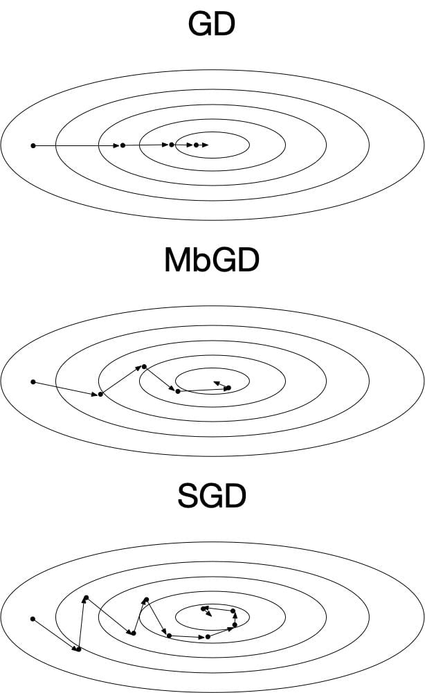
The optimization process difference between the three variants of GD is illustrated in Figure 3. From GD to MBGD and SGD, the updating process becomes noisier and takes more iterations to converge. However, the computation time for each iteration is lower.

Comparison of Teoretical Properties
Here, we investigate the pros and cons for each gradient descent mechanism.
| GD | MbGD | SGD | |
|---|---|---|---|
| Noise in Updates | Low | Mid | High |
| FLOPS/iter | High | Mid | Low |
| RAM usage | High | Mid | Low |
For large datasets such as Image-Net, it is impossible for GD to run on most computers as the memory requirement is extremely large (i.e., you cannot load the entire dataset, $\mathcal{D}$, into RAM).
We might wonder: since SGD only takes low FLOPS/iter but has high gradient noise, will it slow down SGD’s overall convergence?
Researchers have provided the answer (reference) ($k$ represents the algorithm iteration count):
| GD | SGD | |
|---|---|---|
| Convex Function | $\mathcal{O}(\frac{1}{\sqrt{k}})$ | $\mathcal{O}(\frac{1}{\sqrt{k}})$ |
| Lipschitz Gradient + Convex Function | $\mathcal{O}(\frac{1}{k})$ | $\mathcal{O}(\frac{1}{\sqrt{k}})$ |
| Strongly Convex Function | $\mathcal{O}(\gamma^k)$ | $\mathcal{O}(\frac{1}{k})$ |
Here, we measure convergence by $\mathbb{E}[L(\theta^{(k)})-L(\theta^*)]$ in which $\theta^*$ represents the best parameters.
Note that for a loss function $L$ to be convex, the second derivitve with respect to $\theta$ for ALL $\theta$ and $x_i\in \mathcal{D}$ must be positive (for differentible functions), as shown in Equation \ref{second_direvative_greater_than_0}.
\begin{align}
\frac{\partial^2 L(\theta)}{\partial \theta^2}\geq 0,\quad\forall\theta, x_i \in\mathcal{D}
\label{second_direvative_greater_than_0}
\end{align}
Performing GD on convex functions is guaranteed to find the global optimum, $\theta^*$. However, it is generally not guaranteed when functions are non-convex.
Lipschitz Gradient means the gradient of loss $L$ w.r.t. $\theta$ cannot change dramatically locally, as described in Equation \ref{lipschitz_gradient}.
\begin{align}
||\nabla L(\theta)-\nabla L(\theta^\prime)\leq \Omega ||\theta-\theta^\prime||,\quad\exists\Omega,\forall \theta,\theta^\prime
\label{lipschitz_gradient}
\end{align}
Strongly Convex means the function is not only convex but also has at least certain curvature as quadratic functions (reference), as shown in Equation \ref{strongly_convex}.
\begin{align}
\langle\nabla L(\theta)-\nabla L(\theta^\prime),\theta-\theta^\prime\rangle\geq \gamma ||\theta-\theta^\prime||^2,\quad\exists\gamma>0,\forall \theta,\theta^\prime
\label{strongly_convex}
\end{align}
Although these assumptions do not always hold for general loss functions and model choices, we can conclude that SGD’s convergence rate is not as good as GD in the latter two cases, but their convergence is actually the same under convex function assumption! In practice, we cannot say much about the theoretical properties of GD vs SGD, but we at least can go forward knowing that SGD performs comparably on convex functions and is often more feasible when working with Big Data.
Take Away
Although SGD seems to have more noisy updates, SGD’s convergence rate on convex function is the same as GD. Further, SGD requires fewer FLOPS/iter. Therefore, SGD would require fewer total FLOPS to find our best model, $\theta^*$. SGD for the win!
Empirical Comparison
Here, we show an example optimization of the three methods. In line with our theoretical results, they have similar convergence in terms of iterations, and GD > MbGD > SGD in terms of FLOPS.
Note that SGD does have higher noise during the process, and MbGD has similar smooth updates as GD, i.e., the usage of minibatch does help stabilize the update.

Take Away
When the dataset is small, GD is preferred due to its low-noise properties. When the dataset gets large enough, GD becomes infeasible. In this case, SGD is preferred if the data noise is not significant and the noisy updates will not ruin the optimization process, otherwise, MbGD is preferred. We provide our code on Github.
Accelerating GD and SGD
Several variants of GD (such as Momentum GD, RMSProp, Adam) all utilize the core idea of momentum. What is momentum then?
We introduce the initial momentum as
\begin{align}
m^{(0)}=0.
\end{align}
For each iteration, instead of using the gradient to directly update $\theta$, we use the gradient to update the momentum, as shown in Equation \ref{momentum}.
\begin{align}
m^{(i)}=\beta m^{(i-1)}+\nabla_\theta L(\theta^{(i-1)})
\label{momentum}
\end{align}
$\beta\in[0,1)$ is a hyperparameter that you tune, and $\beta=0$ recovers basic GD.
And then use the momentum to update $\theta$ according to Equation \ref{theta_update_momentum}.
\begin{align}
\theta^{(i)}=\theta^{(i-1)}-\alpha m^{(i)}
\label{theta_update_momentum}
\end{align}
What is momentum essentially doing, and when is it useful?
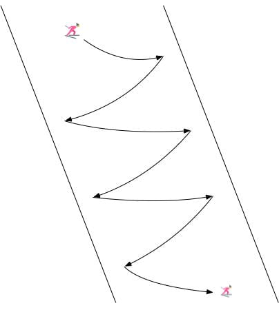
Consider the snowboarding-in-a-half-pipe-like optimization problem depicted in Figure 5.

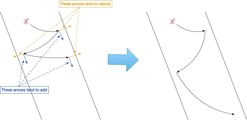
Often in these situations, standard GD will oscillate back and forth because the gradient direction has larger value on vertical direction than horizontal direction. However, we could see that each gradient step still has a small right movement, slowly pushing us to the optimum.
Momentum techniques utilize such phenomenon and gathers the downward forces while canceling out the horizontal forces, resulting as the result shown before.

Another case that momentum helps is when the loss function has a flat region (plateau) as shown in Figure 7.

In this case, gradient descent updates on $\theta$ will get slower in the middle plateau area, even equaling $0$ in extreme cases. However, as long as we accumulate enough momentum before the plateau, we could rush over the plateau, avoiding the small-gradient problem. Momentum can also help push past local minimums so that we can find optimal parameters even if our function is non-convex.
Theoretically, it could be proven that a similar variant of Momentum GD, Nesterov’s accelerated gradient descent, could achieve $O(\frac{1}{k^2})$ convergence instead of $O(\frac{1}{k})$ (reference).
Take Away
Momentum is useful for solving many optimization problems. However, adding momentum in requires extra hyperparameter tuning for $\beta$.
Conclusion
- GD, MbGD, SGD converge at the same rate in terms of iterations.
- SGD requires fewer FLOPS but is noisy.
- Parallization could help MbGD and GD do better in terms of wall clock time.
- Momentum can help but needs careful hyperparameter tuning.
- Many famous optimizers such as Adam use momentum and fancy tricks but it is essentially SGD!
