Zac Chen

Introduction

To solve any machine learning problem we need three ingredients: some data observed in the world, a model to explain our data, and an optimizer that can fit the model to the data. In this blog we re-visit the optimization problem, which we first explained in the Gradient Descent post. We present the problem of constrained optimization and explain the conditions required to achieve an optimal solution when solving constrained optimization problems.

Humans approximately solve constrained optimization problems frequently. For example, if someone wants to find a way to get to the city as quickly as possible without paying highway tolls, that person would be solving a constrained optimization problem. Specifically, the objective is to get to the city as quickly as possible, and the constraint is to not use any roads or highways that might require the person to pay tolls. Such problems are commonplace and require a search over all solutions to verify that the solution is optimal and does not violate any of the constraints. From a computational perspective these constrained optimization problems are NP-hard.

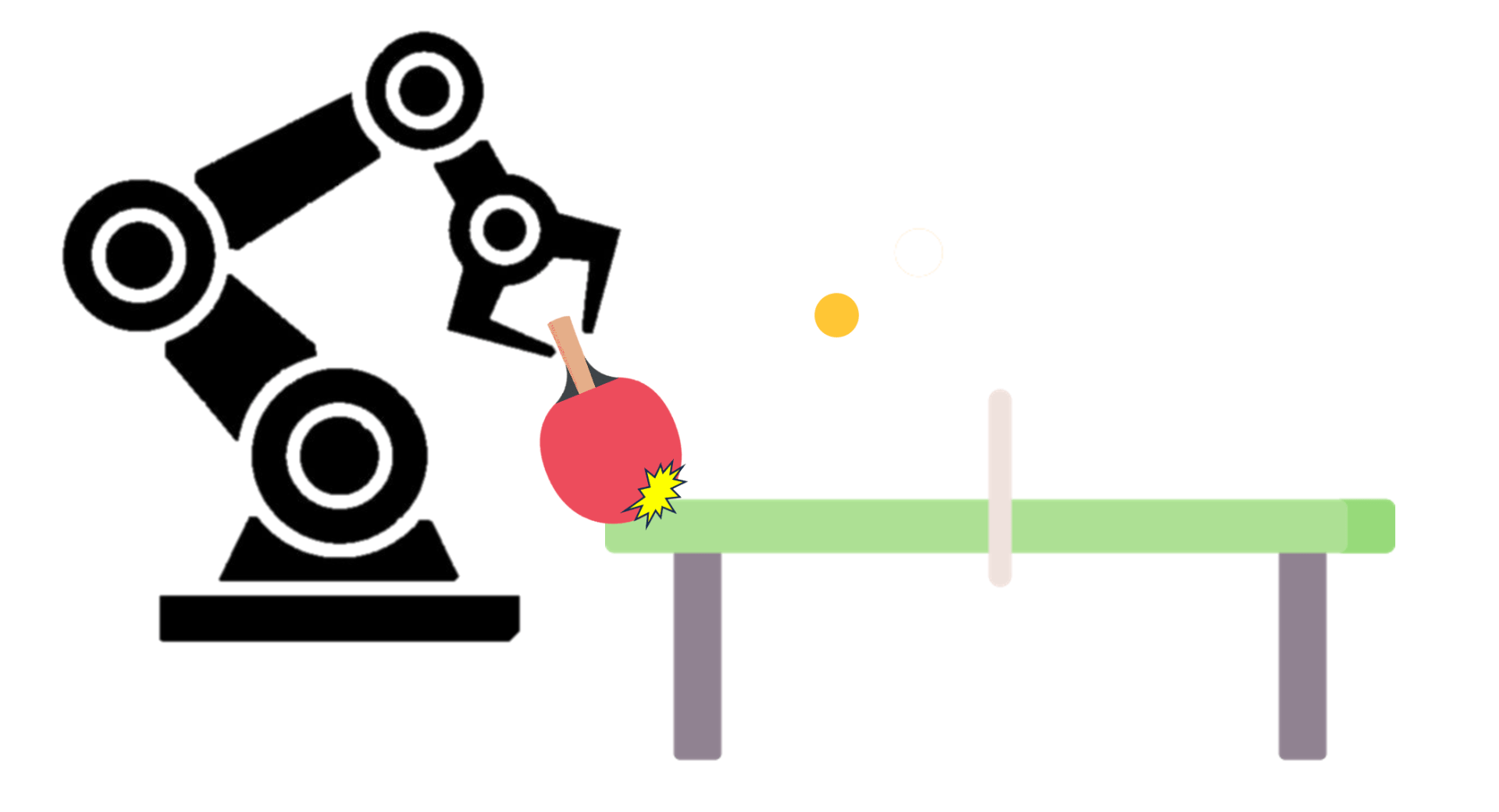
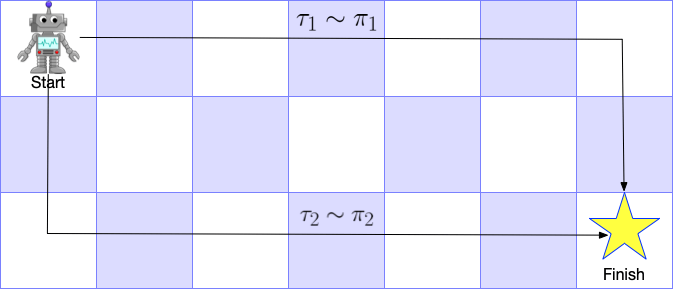
These problems are also present in robot learning. Consider a robot learning to hit a table-tennis ball from demonstrations (Figure 1). We can collect demonstration data of a human moving the robot’s arm through the motion of a table tennis stroke. We might then have a supervised learning model to learn the task by minimizing the distance between the demonstrated and learned robot trajectories. However, there are also several possible constraints to this learning problem. First is a constraint of physics, such as the robot’s forward dynamics model. The forward dynamics model for a robot specifies how much its joints can move under a given force. These can be thought of as equality constraints, $\tau = H(q)\ddot{q}$, where a given torque, $\tau$, specifies the amount a robot joint can move via a joint-space inertia matrix, $H$, whose variables are the robot’s joint angles $q$. Other specific constraints might be that the robot needs to learn these trajectories safely, for example, the robot should never hit the table while playing (Figure 1). This could be done by creating a box around the table and telling the robot to never enter the box. Such a constraint might be an inequality constraint, i.e., $x < 10$, where $x$ is the robot's end-effector position along the $x$-coordinate and at $10m$ might be the edge of the table w.r.t. to the origin of the robot's coordinate frame. Hence the learning problem can have both equality and inequality constraints. Such an optimization problem can be specified as: \begin{alignat*}{3} & \text{minimize}& f(\mathbf{x})\\ & \text{subject to} \quad& h_j(\mathbf{x}) = 0, \forall j\\ & \quad& l_i(\mathbf{x}) \leq 0, \forall i, \label{eq:constrained_optimization} \end{alignat*} where the constraints for the robot's dynamics ($h_j$) and physical space ($l_i$) are specified and the goal would be minimize a loss function for the supervised scenario where the robot generates a table-tennis trajectory similar to the human's demonstration.

Equality Constraints in a learning problem

We first examine the solution to the constrained optimization problem considering only equality constraints. Consider the problem of form:
\begin{alignat}{3}
& \text{minimize} \quad f(x_1,x_2) \nonumber \\
& \text{subject to} \quad h_0(x_1,x_2) = c \quad .
\end{alignat}

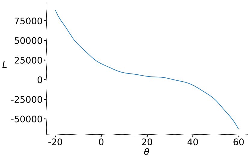
In this example vector $\mathbf{x} = [x_1,x_2]$, and there is only one constraint $h_0$. Figure 2 provides an example function $f(\mathbf{x})$, and its equality constraint $h(\mathbf{x})$. Notice that the optimal point for the function under the constraint is a point where the constraint function is tangent to the isoline with value $d_1$. This is because moving along the equality constraint does not make the values of the function $f(\mathbf{x})$ increase in either direction, meaning that this is a stationary point. An optimal value of the function under constraints can only exist on such stationary points. This stationarity condition is a necessary condition for optimality. Further, the gradient of the function is parallel to the gradient of the equality constraint, as the two curves, i.e, the optimization function and constraint, are tangent at these stationary points. If the two curves are tangent, their gradients vectors differ only by a scalar, i.e., $\nabla f = \lambda \nabla h$. This property is shown in Figure 2 more clearly.

The Lagrangian function can then be defined as:
\begin{equation}
\mathcal{L}(\mathbf{x},\lambda) = f(\mathbf{x}) + \lambda h(\mathbf{x}),
\end{equation}
where the necessary, but not sufficient, condition for optimality is $\nabla_{\mathbf{x}, \lambda} \mathcal{L}(\mathbf{x}, \lambda) = 0$. We can now use gradient descent to find a locally optimal solution for the Lagrangian function, which will provide us with solution for both, the parameter $\lambda$, and values for the vector $\mathbf{x}$ for the locally optimal solution. If the two functions, $f$ and $h$ are convex, then the solution will be a globally optimal solution. This technique of converting a constrained optimization problem into the new function where the constraints are summed is called the Lagrange multipliers technique. The Lagrange multipliers technique hence allows us to use gradient descent to solve a constrained optimization problem, which allows for a computationally feasible way to solve these problems, without the use of matrix inversions.

Inequality constraints in the optimization problem

To solve constrained optimization problems with inequality constraints, we again use Lagrangian multipliers. Consider the following constrained optimization problem:
\begin{alignat}{3}
& \text{minimize}& f(\mathbf{x}) \nonumber \\
& \text{subject to} \quad& h_j(\mathbf{x}) = 0, \forall j \nonumber \\
& \quad& l_i(\mathbf{x}) \leq 0, \forall i
\end{alignat}
This is the primal problem, where we are minimizing the function w.r.t. to the input variable $\mathbf{x}$. However, a dual problem can be formulated, which is maximized w.r.t. to the constraint variables. Sometimes the dual problem might make the primal problem computationally tractable, or vice versa, because the evaluation in one of the forms for the function being computed might be easier.

A dual problem changes the variables of the optimization problem and the direction of the optimization from a minimization problem to a maximization problem. The value of the primal and the dual problem at the optimal solution are equal, where the minimization problem provides the upper bound, and the maximization problem, i.e., the dual, presents the lower bound for the values of the primal problem.
We formulate the dual with the Lagrangian:
\begin{equation}
\mathcal{L}(\mathbf{x},\mathbf{\lambda},\mathbf{\alpha}) = f(\mathbf{x}) + \sum_j \lambda_j h_j(\mathbf{x}), + \sum_i \alpha_j l_i(\mathbf{x}).
\end{equation}
The dual function using this Lagrangian would be:
\begin{equation}
g(\mathbf{\lambda},\mathbf{\alpha}) = \textrm{min}_x \mathcal{L}(\mathbf{x},\mathbf{\lambda},\mathbf{\alpha}),
\end{equation}
and the dual optimization problem would be:
\begin{alignat}{3}
\lambda^*\!, \alpha^* =& \text{argmax}_{\mathbf{\lambda}, \mathbf{\alpha}} g(\mathbf{\lambda}, \mathbf{\alpha}) \nonumber \\
& \alpha_i \geq 0, \forall i .
\label{eq:dual_prob}
\end{alignat}

To find the optimal solution for the constrained optimization problem we need to find values of $\mathbf{x},\mathbf{\lambda},\mathbf{\alpha}$ at which the Lagrangian is stationary, and both the primal and dual problems are satisfied without any constraint violations. We use gradient descent iteratively to solve this problem:

[Step 1] Find the optimal value of $\mathbf{x}$ under which the Lagrangian is minimized, i.e, $\mathbf{x}* = \textrm{argmin}_{\mathbf{x}} \mathcal{L}(\mathbf{x},\mathbf{\lambda},\mathbf{\alpha})$. We pick the values for $\mathbf{\lambda}$ and $\mathbf{\alpha}$ at random for the first iteration.

[Step 2] Holding the optimal value of $\mathbf{x}*$ found previously, we now find the gradient of $\mathcal{L}$ w.r.t. $\mathbf{\lambda}$ and $\mathbf{\alpha}$, and update their values with a learning rate to perform gradient ascent. This is akin to moving slowly towards the optimal solution of the dual problem defined in Eq. \ref{eq:dual_prob}.

We iterate over both these steps until we reach the stopping conditions, which are called the Karush–Kuhn–Tucker (KKT) conditions for optimality. These conditions are:

1. Stationarity: The gradient of the Lagrangian is zero as explained in the previous section, i.e., $\nabla \mathcal{L} = 0$.
2. Primal feasiblity: The constraints of the primal problem are satisfied, i.e., $h_j(\mathbf{x}) = 0, \forall j,$ and $l_i(\mathbf{x}) \leq 0, \forall i$.
3. Dual feasiblity: The constraints of the dual problem are satisfied, i.e., $\alpha_i \geq 0, \forall i$.
4. Complimentary Slackness: $\sum_i \alpha_j l_i(\mathbf{x}) = 0$. This ensures that either the inequality constraints in the primal are satisfied by equality, i.e., are tight, and $\alpha_i$ is unbounded, or $\alpha_i = 0$, and the constraint has a lot more slack in satisfiability.

The KKT conditions provide the necessary conditions for local optimality for a constrained optimization problem with inequality constraints. These conditions were developed as a generalization to the Lagrange Multipliers technique that account for both equality and inequality constraints. The Lagrange multipliers technique developed in the previous section is a technique only applicable to equality constraints.

We can compute the solution of the primal and the dual at each iteration of the optimization problem, and also compute the optimality gap: $\frac{p^k-d^k}{d^k}$, where $p^k$ and $d^k$ are the values of the primal and dual problems in iteration $k$ of the optimization. Here the solution of the minimization primal problem provides the upper bound of the function value and the solution of the dual provides the lower bound of the function value, which converge towards each other asymptotically over optimization iterations. The optimality gap provides a range within which the optimal constrained solution lies and gives us an upper and lower bound over our solution quality.

Key Takeaways

1. Constrained optimization is an important and computationally challenging problem needed for robot and machine learning.
2. Given a constrained optimization problem, a Lagrangian can be formulated where the constraints are used as additive factors to the optimization function. The stationary points of the Lagrangian are candidates for the optimal solution of the optimization problem.
3. The Lagrange multipliers technique allows us to use gradient descent to solve a constrained optimization problem, which allows for a computationally feasible way to solve these problems by avoiding matrix inversions. These solution methods take a different form to solve approximately for non-convex problems which are generally faster.
4. Karush–Kuhn–Tucker (KKT) conditions provide the necessary conditions for local optimality for a constrained optimization problem with inequality constraints. These conditions were developed as a generalization to the Lagrange Multipliers technique.

Gradient Descent (GD) is an intuitive optimization method. GD has become one of the most popular optimization methods in recent years due to its nice theoretical properties, effectiveness in real-world applications, and uncanny ability to train large-scale deep learning models. GD is commonly used in deep learning for finding neural network parameters that best capture patterns in the data. In this blog, we introduce three different flavors of GD, regular GD, Stochastic GD (SGD), and Minibatch GD (MbGD). We analyze these variants theoretically as well as empirically, and discuss which one is most appropriate for different scenarios! Finally, we discuss how GD can be improved or “accelerated” by adding “momentum”.

This blog is divided into four parts:

1. Introduction of GD, SGD, and MbGD
2. Analytical results
3. Empirical results
4. Accelerated GD

What is GD, SGD, and MbGD?

Let’s first look at a simple machine learning scenario. We have a dataset $\mathcal{D}=\{(x_i,y_i),\ i\in [n]\}$, where $(x_i,y_i)$ is  “example” number $i$, $x_i$ is the input to a model we want to train and $y_i$ is the “label” we want our model to learn to predict from $x_i$. For instance, $x_i$ might be the date of the year, and $y_i$ might be the expected rainfall you would receive that day. In this simplified example, we assume $x_i$ is a scalar instead of a vector, but the concept and the math work for the vector case (where $x_i$ contains several features) too.

To allow us to visualize the model, let’s assume we are using a linear model parameterized by $\theta$ shown in Equation \ref{f}.
\begin{align}
f_\theta(x_i)=\theta x_i
\label{f}
\end{align}
The metric we use to judge our model (i.e., a “loss function”) is the Mean Squared Error (MSE) loss (Equation \ref{L}), which calculates the squared error for each prediction and averages over all data points.
\begin{align}
L(\theta)=-\frac{1}{2n}\sum_{i=1}^n(y_i-f_\theta(x_i))^2
\label{L}
\end{align}
We want to find the best model, $\theta^*$, according to our loss function (Equation \ref{loss}).
\begin{align}
\theta^*=\arg\min_\theta L(\theta)
\label{loss}
\end{align}

\(L\) is a quadratic function of the model parameter \(\theta\), illustrated in Figure 1. The problem then is to find the critical point, $\theta^*$, that is located at the minimum of this curve. To find the critical point, we set the first derivative of $L$ equals to $0$, i.e. $\frac{\partial L(\theta)}{\partial \theta}=0$. In the case of a simple linear model, we can directly solve for model parameters $\theta^*$. However, in deep learning, such direct methods do not exist. Instead, we need something else. In this tutorial, that “something else” is GD.

GD

In GD, we perform three steps:

1. Calculate the gradient of our model parameters.
2. Use the gradient to update model parameters.
3. Repeat steps 1 and 2 until a pre-set tolerance is achieved.

We use $\nabla$ as the gradient operator and it is defined in Equation \ref{gradient}.
\begin{align}
\nabla_\theta=\left[\begin{matrix}
\frac{\partial}{\partial \theta_1}\\
\frac{\partial}{\partial \theta_2}\\
\cdots\\
\frac{\partial}{\partial \theta_m}\\
\end{matrix}\right]
\label{gradient}
\end{align}
First, we calculate the gradient of $L$ w.r.t. $\theta$ in MSE loss (Equation \ref{L}), shown in Equation \ref{gradient_of_L}.
\begin{align}
\nabla_\theta L=-\frac{1}{n}\sum_{i=1}^n(y_i-f_\theta(x_i))\nabla_\theta f_\theta(x_i)\bigg\rvert_{x_i}
\label{gradient_of_L}
\end{align}
In our case of linear model (Equation \ref{f}), we could write the gradient as in Equation \ref{L_linear}.
\begin{align}
\begin{split}
\nabla_\theta L&=-\frac{1}{n}\sum_{i=1}^n(y_i-\theta x_i)x_i\\
&=\frac{1}{n}\sum_{i=1}^nx_i^2\theta-\frac{1}{n}\sum_{i=1}^nx_iy_i
\end{split}
\label{L_linear}
\end{align}
The gradient $\nabla_\theta L$ is a linear function of $\theta$, as shown in Figure 2.

Second, we would like to use the calculated gradient to update our model parameters. As we want to minimize the loss function, GD follows the negative gradient direction. We update our parameters by this gradient multiplied by a small step size $\alpha$ (a hyperparameter), as shown in Equation \ref{negative_gradient_step}.
\begin{align}
\theta^{(i)}\leftarrow \theta^{(i-1)}-\alpha \nabla_\theta L(\theta^{(i-1)})
\label{negative_gradient_step}
\end{align}
Empirically, we choose $\alpha$ to be ${10}^{-5}-{10}^{-3}$. Utilizing an $\alpha$ value that is too small will result in slower learning and require more iterations of (1) and (2). An $\alpha$ value that is too large may be even more detrimental. It may lead to behavior that causes the model parameters $\theta$ to oscillate or even diverge.

Finally, GD continues to iterate until a pre-set tolerance is achieved (norm of gradient is small, function value is small, or iteration number is large, etc).

If the function to be optimized (in our case, the loss function, $L$) is convex w.r.t. the parameters $\theta$, GD is guaranteed to converge to a global minimum given alpha is small enough. However, if this assumption does not hold, the model parameters could become stuck in a local minimum of the loss function $L$. For problems that are non-convex, we often perform GD several times with sets of randomly initialized theta, hoping to find the global minimum.

Why take the negative gradient direction?

In order to minimize the loss in Figure 1, we look at two cases: where $\theta >4.5$ and $\theta < 4.5$. If $\theta$ is greater than $4.5$, we need to move left along the loss curve to decrease our loss value. If $\theta$ is less than $4.5$, we should move right.

From Figure 2, we can see that $\nabla_\theta L>0$ when $\theta>4.5$ and $\nabla_\theta L <0$ when $\theta<4.5$. Utilizing the negative of these gradients in our update rules allows us to improve theta, i.e. decreases our loss function.

This idea of “taking a step” comes from using a first order Taylor Expansion of $L(\theta)$, mathematically shown in Equation \ref{taylor_expansion}.
\begin{align}
L(\theta^\prime)\approx L(\theta)+(\theta^\prime-\theta)\nabla_\theta L(\theta)
\label{taylor_expansion}
\end{align}
Therefore, if our goal is to make $L(\theta^\prime)$ smaller, we can take $\theta^\prime=\theta-\alpha\nabla_\theta L(\theta)$, as
\begin{align}
\begin{split}
L(\theta-\alpha\nabla_\theta L(\theta))&\approx L(\theta)-\alpha\nabla_\theta L(\theta)\nabla_\theta L(\theta) \\
&= L(\theta)-\alpha(\nabla_\theta L(\theta))^2\\
&< L(\theta).\quad ((\nabla_\theta L(\theta))^2\geq 0, \alpha>0)
\end{split}
\end{align}

Accordingly, GD is guaranteed to reduce the loss function if $\alpha$ is infinitely small. As a result, GD will go down the hill, as shown in Figure 1.

SGD

Stochastic Gradient Descent (SGD) has one fundamental difference compared to standard GD: instead of using the entire dataset to calculate the gradient $\nabla_\theta L$ in each step, we sample only one data point from the dataset and use that specific data to calculate $\nabla_\theta L$. Speficaly, in our example, the gradient of the loss function computed over one datapoint is shown in Equation \ref{gradient_SGD}.
\begin{align}
\begin{split}
\nabla_\theta L(\theta^{(i-1)})&=-(y_j-\theta^{(i-1)} x_j) x_j\\
&=x_j^2\theta^{(i-1)}-x_jy_j\\
& j\sim \mathcal{U}\{1,n\}
\end{split}
\label{gradient_SGD}
\end{align}
Here, $\mathcal{U}\{1,n\}$ represents discrete uniform distribution.

Because we only compute our gradient update for one data point, SGD requires less computation (Floating Point Operations Per Second, FLOPS) than GD in each iteration. However, since we are calculating the gradient from just one sample of data, and the data may be noise (typical in real-world datasets), SGD may take steps in the wrong direction.

MbGD

Minibatch Gradient Descent represents a middle ground between GD and SGD, sampling a small subset of examples from our dataset to calculate $\nabla_\theta L$:
\begin{align}
\begin{split}
\nabla_\theta L(\theta^{(i-1)})&=-\frac{1}{n^\prime}\sum_{j\in\mathcal{B^{(i)}}}(y_j-\theta^{(i-1)} x_j) x_j\\
&=\frac{1}{n^\prime}\sum_{j\in\mathcal{B^{(i)}}}x_j^2\theta^{(i-1)}-x_jy_j
\end{split}
\end{align}
In this equation, $\mathcal{B}=\{i_1,\cdots,i_{n^\prime}\}, i_j\sim \mathcal{U}\{1,n\}$. $n^\prime$ is the size of the minibatch. The size of minibatch is a hyperparameter you choose.

Visualization of GD, MbGD and SGD

The optimization process difference between the three variants of GD is illustrated in Figure 3. From GD to MBGD and SGD, the updating process becomes noisier and takes more iterations to converge. However, the computation time for each iteration is lower.

Comparison of Teoretical Properties

Here, we investigate the pros and cons for each gradient descent mechanism.

This table summarizes pros and cons of each GD variant.

	GD	MbGD	SGD
Noise in Updates	Low	Mid	High
FLOPS/iter	High	Mid	Low
RAM usage	High	Mid	Low

For large datasets such as Image-Net, it is impossible for GD to run on most computers as the memory requirement is extremely large (i.e., you cannot load the entire dataset, $\mathcal{D}$, into RAM).

We might wonder: since SGD only takes low FLOPS/iter but has high gradient noise, will it slow down SGD’s overall convergence?

Researchers have provided the answer (reference) ($k$ represents the algorithm iteration count):

This table displays the convergence rate of each GD variant under different assumptions.

	GD	SGD
Convex Function	$\mathcal{O}(\frac{1}{\sqrt{k}})$	$\mathcal{O}(\frac{1}{\sqrt{k}})$
Lipschitz Gradient + Convex Function	$\mathcal{O}(\frac{1}{k})$	$\mathcal{O}(\frac{1}{\sqrt{k}})$
Strongly Convex Function	$\mathcal{O}(\gamma^k)$	$\mathcal{O}(\frac{1}{k})$

Here, we measure convergence by $\mathbb{E}[L(\theta^{(k)})-L(\theta^*)]$ in which $\theta^*$ represents the best parameters.

Note that for a loss function $L$ to be convex, the second derivitve with respect to $\theta$ for ALL $\theta$ and $x_i\in \mathcal{D}$ must be positive (for differentible functions), as shown in Equation \ref{second_direvative_greater_than_0}.
\begin{align}
\frac{\partial^2 L(\theta)}{\partial \theta^2}\geq 0,\quad\forall\theta, x_i \in\mathcal{D}
\label{second_direvative_greater_than_0}
\end{align}
Performing GD on convex functions is guaranteed to find the global optimum, $\theta^*$. However, it is generally not guaranteed when functions are non-convex.

Lipschitz Gradient means the gradient of loss $L$ w.r.t. $\theta$ cannot change dramatically locally, as described in Equation \ref{lipschitz_gradient}.
\begin{align}
||\nabla L(\theta)-\nabla L(\theta^\prime)\leq \Omega ||\theta-\theta^\prime||,\quad\exists\Omega,\forall \theta,\theta^\prime
\label{lipschitz_gradient}
\end{align}

Strongly Convex means the function is not only convex but also has at least certain curvature as quadratic functions (reference), as shown in Equation \ref{strongly_convex}.
\begin{align}
\langle\nabla L(\theta)-\nabla L(\theta^\prime),\theta-\theta^\prime\rangle\geq \gamma ||\theta-\theta^\prime||^2,\quad\exists\gamma>0,\forall \theta,\theta^\prime
\label{strongly_convex}
\end{align}

Although these assumptions do not always hold for general loss functions and model choices, we can conclude that SGD’s convergence rate is not as good as GD in the latter two cases, but their convergence is actually the same under convex function assumption! In practice, we cannot say much about the theoretical properties of GD vs SGD, but we at least can go forward knowing that SGD performs comparably on convex functions and is often more feasible when working with Big Data.

Take Away

Although SGD seems to have more noisy updates, SGD’s convergence rate on convex function is the same as GD. Further, SGD requires fewer FLOPS/iter. Therefore, SGD would require fewer total FLOPS to find our best model, $\theta^*$. SGD for the win!

Empirical Comparison

Here, we show an example optimization of the three methods. In line with our theoretical results, they have similar convergence in terms of iterations, and GD > MbGD > SGD in terms of FLOPS.

Note that SGD does have higher noise during the process, and MbGD has similar smooth updates as GD, i.e., the usage of minibatch does help stabilize the update.

Take Away

When the dataset is small, GD is preferred due to its low-noise properties. When the dataset gets large enough, GD becomes infeasible. In this case, SGD is preferred if the data noise is not significant and the noisy updates will not ruin the optimization process, otherwise, MbGD is preferred. We provide our code on Github.

Accelerating GD and SGD

Several variants of GD (such as Momentum GD, RMSProp, Adam) all utilize the core idea of momentum. What is momentum then?

We introduce the initial momentum as
\begin{align}
m^{(0)}=0.
\end{align}

For each iteration, instead of using the gradient to directly update $\theta$, we use the gradient to update the momentum, as shown in Equation \ref{momentum}.
\begin{align}
m^{(i)}=\beta m^{(i-1)}+\nabla_\theta L(\theta^{(i-1)})
\label{momentum}
\end{align}
$\beta\in[0,1)$ is a hyperparameter that you tune, and $\beta=0$ recovers basic GD.
And then use the momentum to update $\theta$ according to Equation \ref{theta_update_momentum}.
\begin{align}
\theta^{(i)}=\theta^{(i-1)}-\alpha m^{(i)}
\label{theta_update_momentum}
\end{align}

What is momentum essentially doing, and when is it useful?

Consider the snowboarding-in-a-half-pipe-like optimization problem depicted in Figure 5.

Often in these situations, standard GD will oscillate back and forth because the gradient direction has larger value on vertical direction than horizontal direction. However, we could see that each gradient step still has a small right movement, slowly pushing us to the optimum.

Momentum techniques utilize such phenomenon and gathers the downward forces while canceling out the horizontal forces, resulting as the result shown before.

Another case that momentum helps is when the loss function has a flat region (plateau) as shown in Figure 7.

In this case, gradient descent updates on $\theta$ will get slower in the middle plateau area, even equaling $0$ in extreme cases. However, as long as we accumulate enough momentum before the plateau, we could rush over the plateau, avoiding the small-gradient problem. Momentum can also help push past local minimums so that we can find optimal parameters even if our function is non-convex.

Theoretically, it could be proven that a similar variant of Momentum GD, Nesterov’s accelerated gradient descent, could achieve $O(\frac{1}{k^2})$ convergence instead of $O(\frac{1}{k})$ (reference).

Take Away

Momentum is useful for solving many optimization problems. However, adding momentum in requires extra hyperparameter tuning for $\beta$.

Conclusion

1. GD, MbGD, SGD converge at the same rate in terms of iterations.
2. SGD requires fewer FLOPS but is noisy.
3. Parallization could help MbGD and GD do better in terms of wall clock time.
4. Momentum can help but needs careful hyperparameter tuning.
5. Many famous optimizers such as Adam use momentum and fancy tricks but it is essentially SGD!