• Skip to primary navigation
  • Skip to content
  • Skip to primary sidebar
  • Skip to secondary sidebar

CORE Robotics Lab

  • Home
  • Publications
  • People
  • Robots
  • Blog
  • Contact Us

Manisha Natarajan

Presentation Guidelines for PhD Proposal

June 13, 2023 by Batuhan Altundas, Arthur Scaquetti do Nascimento, Manisha Natarajan and Matthew Gombolay

Presenting your PhD Thesis Proposal is an exciting step in your PhD journey. At this point, you will have formed your PhD committee, developed initial results (potentially published one or more papers as the foundation to your proposal), and formulated a plan for conducting your proposed research. Many students can find the proposal experience stressful. In a sense, the proposal defines the “story” you will tell for years to come, including at your Thesis Defense, faculty job talks, and beyond. However, it is important to focus on the here and now rather than getting wrapped up in the expectations for the future and so many things that are outside of your control. Try to focus on what you can control and do the best you can to deliver a high-quality proposal.

This blog is a guide to help you do that — give a high-quality proposal presentation. This guide omits much about how to give a talk in general and instead focuses on common issues that come up specifically at the PhD Proposal Presentation stage of one’s academic development. For many, this may be the first time you will be presenting to an audience of professors your prior work and a proposal for what you will accomplish in a longform (e.g., 45-50 minutes) talk and be expected to defend your plan for an additional 45-50 minutes. Remember, the Committee’s job is to critique your work and challenge you into a better Thesis direction, to make your research better. Expect to be challenged and for your proposed work to change coming out of the proposal — this is a good thing 🙂

Having said all that, here is a non-exhaustive list of tips in three sections: Before, During, and After (i.e., the Q&A session) the proposal presentation.

Before The Proposal

1) Meet Committee Members a priori

Interviewing your Committee members before your Proposal is a great way to get to know them personally and allow you to assess the compatibility of the Committee Candidate and yourself. Share with them a compressed thesis pitch and get their feedback (include the proposed Thesis Statement from Point 2 below). If there appears to be an irreconcilable issue with your proposed work, you should both (1) consider the feedback you received with your PhD advisor to see if you can make the proposal better and (2) consider whether that committee member might present an insurmountable critic for you in successfully defending. Not everyone will like your work — that is ok. Just try to learn from every critic to see if you can make your proposal sharper.

After selecting your committee, meet with each member before the Proposal Presentation to ask if you are ready to Propose. That will give you a good indication (and hopefully lead to more profound feedback) of the level of critique of your work, as well as their expectations for improvements.

  • It allows you to get comfortable with them, making the Proposal presentation less stressful.
  • It gives you an opportunity to present the work to your Committee Members and give them an overview of what they can expect from the Proposal.
  • If they support you going through with presenting your Proposal, they are more likely to support you during the Proposal and vote in your favor. If they state that your work is not ready to be proposed, they can also offer suggestions to improve it and ensure that you are ready to  propose.
  • It allows the student to get a sneak peek at questions the Committee Members may ask during the Proposal and gives you time to prepare answers.

During The Proposal

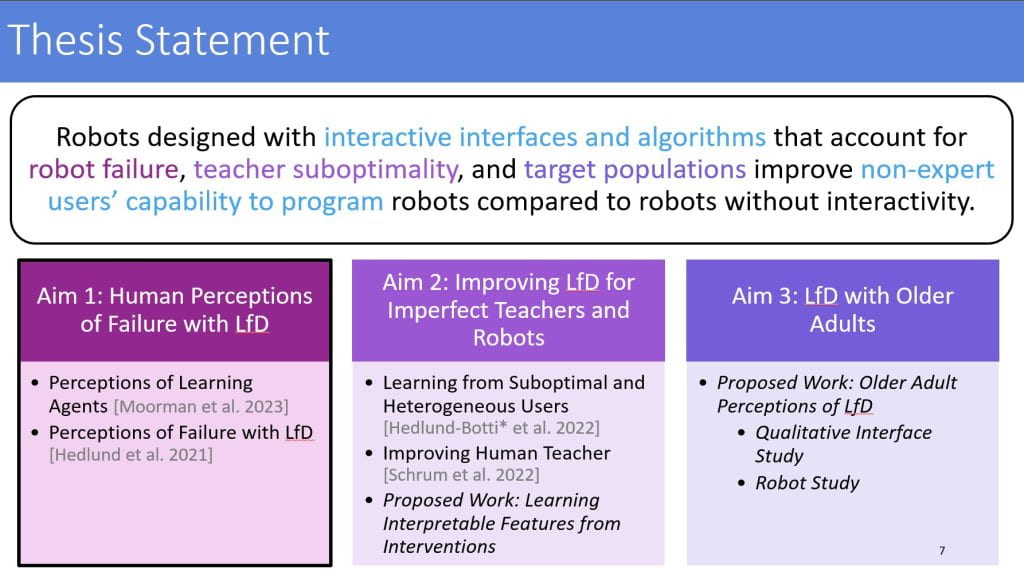
2) Have a clear Thesis Statement

  • Present the thesis statement before going over your research and at the end, tying everything together with that “golden” paragraph.
  • A Thesis Statement should be nonobvious. Always remember that the proposal should set up the proposed research, experiments, and analysis. These components will serve as the supporting arguments and evidence in favor of your Thesis Statement.
  • Be mindful that your Thesis’ scope presented in your Proposal is subject to change based on feedback from the Committee. The purpose of clearly laying a Thesis Statement is to show that you are working towards a cohesive topic.

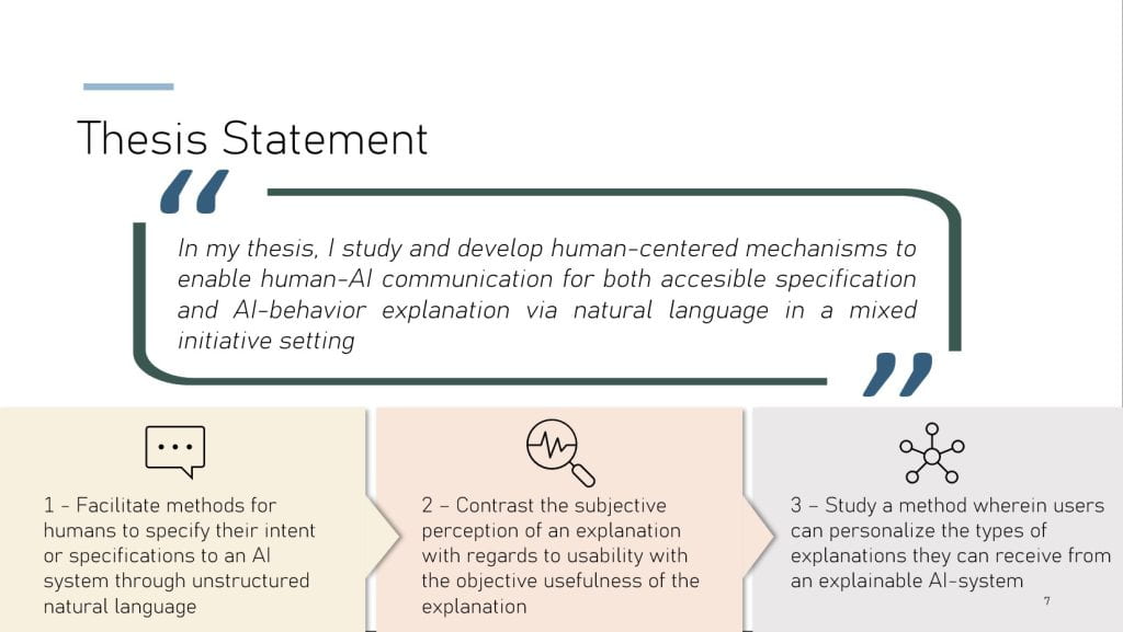
    Figure 1: Sample Slide from Pradyumna Tambwekar’s Proposal. The student shows a clear statement early in the presentation, and breaks it down into the main steps, which will serve as his roadmap.

3) Have a Venn Diagram of the Literature Review

Every proposal needs to present to the committee a review of the relevant literature. The proposer needs to convey that the proposer has assimilated a representative set of knowledge from prior work and that the proposed work is novel and significant. A Venn Diagram of the research based on topics is a good method of presenting prior work and situating your proposed work within this sea of prior work.  Typically, your Thesis will be at the intersection of multiple (sub-)fields, and your work would lie at the intersection. Here are some advantages of this diagram:

  • Having a Venn Diagram of previous literature, and where your own previous and future works fall into shows that you have done your literature review, have worked on topics related to these research and how your work fits in the broad scope of the fields.
  • It showcases the novelties that you are bringing to the research committee. Most theses combine multiple topics into a cohesive whole and address a problem that had not been addressed, or use an approach that has not been used in the past.
  • It makes your committee have more confidence in your work given your understanding of relevant literature and how your scientific production fit in to the field.
Figure 2: Sample Slide from Esmaeil Seraj’s Proposal. The Venn Diagram shows the previous work that has been conducted in a field, how the student’s work up to the proposal fits into these fields of research, which areas of interaction exists, and where the proposed work will fit in.

Pro Tip: While a Venn Diagram is a good starting point, you can consider variations.

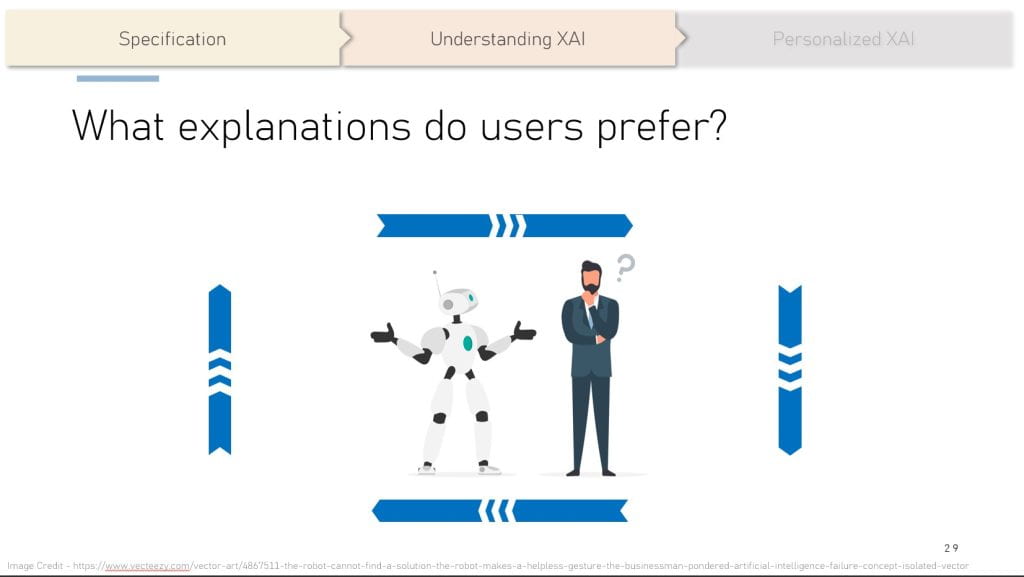
4) Reminders, scaffolds, and roadmaps

The flow of your presentation must be smooth, and this is a great technique to let the audience know how things are connected and whether you are done with a point, or still talking about it. Jumping from topic to topic would get your audience confused. Each work should be linked to the Thesis Statement and ideally to each other. Make sure you verbally and graphically tell the audience when you are switching from one topic to another, and how they relate (in case they do).

  • Roadmap: Your Thesis should hold cohesion, a story that you can refer to as you progress through your presentation. A roadmap is an overview of the steps, aims, and previous research you have conducted that make up your work. These are the parts that make up your Thesis. The purpose of the roadmap is to allow for a smooth flow of your presentation and a method for your Committee to evaluate each work with respect to the whole.
  • Scaffolding: Before presenting each research aim, refer back to the Thesis Statement and previous research you have done, point out what needs to be addressed next and how it relates to the next research aim you are going to present.
  • Reminders: Once each section of your research is complete, refer back to your Thesis statement, explain how what you have presented fits into the broader scope of your Thesis, and re-emphasize your Thesis Statement.

Consider the example outline slide shown below (Figures 1-2) that combines a presentation overview and elements of a thesis statement that would appear throughout the presentation to transition between sections.

Figure 3: Sample Slide from Esmaeil Seraj’s PhD Defense, where the Thesis Statement is structured around research conducted prior to the proposal (in blue and green) and research conducted after the proposal (in red).


Figure 4: Sample Slide from Pradyumna Tambwekar’s Proposal. Notice how the student keeps track of the topics that were already covered on the top of the page.

5) Acknowledge collaboration

It is likely that you have worked with others when doing research. Be clear on who has done what and assign credit where it is due as you go through each of your research aims, preventing possible accusations of plagiarism. Acknowledge second authorship (i.e. “in this study led by Jane Doe, we looked into…”). Collaboration is not a bad thing! You just need to acknowledge it up front.

6) The Art of Story Telling (Your Technical Deep-dive)

The best stories have one nadir or low-point. In a story like Cinderella, the low-point is typically sad, coinciding with the protagonist’s efforts having fallen apart. However, in the PhD thesis proposal, you can think of this point as the opportunity for the deepest technical dive in your talk.  Typically, an audience has a hard time handling multiple deep-dives — humans can only pay attention hard enough to understand challenging, technical content about once in a talk. Proposals that start with the low-level technical details and stay low-level for the next hour are going to cause your audience to have their eyes glaze over.

Note: You can also think of the beginning of the story as either an exciting motivation (like Man In Hole or Boy Meets Girl) or a motivation based upon a tragic or scary problem that your research is trying to address (e.g., like Cinderella). This point deserves its own whole blog post! Stay tuned 🙂

Basic Plots: Vonnegut's Cinderella | Story Empire
Figure 5: Image courtesy: https://storyempire.com/2021/02/12/basic-plots-vonneguts-cinderella/.

7) Modulate your voice and body language

Just like the entire presentation tells a story, think of each slide as telling a story. Your voice and body language can do a lot to help the audience follow the argument you are trying to make.

  • Use your steps around the room to help with your pacing (it is often helpful to sync your voice with your steps).
  • Use dramatic pauses (and stop walking) after each argument or punchline – that helps the audience to absorb your point or catch up with the train of thought.
  • Upspeak can be helpful to show enthusiasm in between points, but be mindful that its overuse could be perceived as a lack of confidence.
  • Breathe from your diaphragm.
  • Other voice dynamics techniques can be useful.

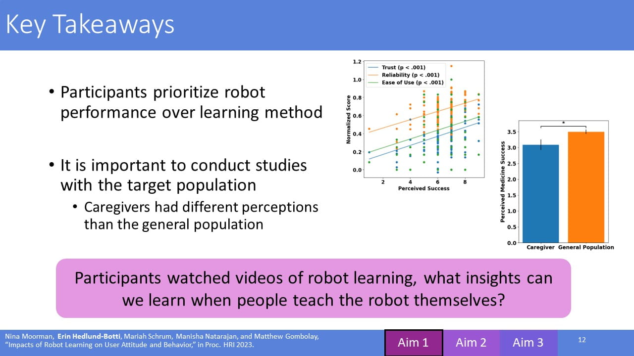
8) Talk about everything on your slide

If you have content on your slide, your audience will want to understand it. If you do not explain it, that will frustrate your audience. Please take the time to talk through everything on your slide. If you don’t want to talk about it, then perhaps you shouldn’t have it on the slide to begin with!

If you have a lot of content on a slide, use animations to control when piece of text or figures pop up on your slides. Otherwise, your committee may start paying attention to the slide to understand the myriad of content and ultimately ignore everything you are saying. Animations are your friend for complex slides. Use animations (or sequences of “build-up” slides) to get the timing right so that your voice and the slide visuals are synergistic. Though, please note that animations can become cheeky, so don’t go overboard.

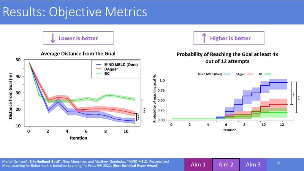
A key issue here is that proposer often forgets to explain all figures and plot axes. Your committee will not instantly understand a figure even though it is a visual. Describe the metrics used, go through the legend, and detail every aspect of the plot so that each member of the audience can see the patterns you want them to recognize.

In summary, you need to:

  • Convey clarity and transparency.
  • Define and explain the axes and metrics.
  • Make it clear whether higher or lower is better for each figure.
  • Note: explaining a figure helps with controlling your own pacing and locking the attention of the audience. Use that moment to re-calibrate it.
Figure 6: Sample Slide from Erin Hedlund-Botti’s Proposal. Notice that all axes are labeled, and all the important information is highlighted. Moreover, the bottom of the slide touches on tip #4. Note that the use of titles in figures is a arguable point, but it is important to include a title or other distinguishing feature when you have multiple figures on a single slide.

9) Have takeaways or “bumpers” on your slides

Clearly show what the scientific novelties/engineering advances of your work are and why it is worth doing what you are doing. This is the part where salesmanship comes in. Answer the following questions:

  • What is the Scientific Impact/Advancement?
  • Where does it stand with respect to prior literature and how is it novel?
Figure 7: Sample Slide from Erin Hedlund-Botti’s Proposal. The student has Key Takeaways for each of the aims presented in the Proposal. This also acts as a recap and preparation for the next topic that will be introduced.

10) Have a Timeline and a List of Planned Publications

A Proposal is a plan for the future that your Committee can look into and suggest changes going forward to the final stretch of the Thesis. As such, a timeline in the form of a Gantt Chart, along with a list of Planned Publications would provide a greater insight on what the Proposed work will be and how it will be done.

The planned work acts as a preview of what the Committee can expect from the Thesis Defense and when it will take place. It also allows them to assess both the quality and feasibility of the proposed work.

Figure 8: Sample Slide from Erin Hedlund-Botti’s Proposal showing the timeline through the published works.

After The Proposal Presentation (The Q&A Session)

11) First things first…

  • Repeat the question back for the sake of the audience.
    • It allows the audience to pay attention to the question being answered if they have not heard it at first.
    • It gives you time to think over an answer.
    • It allows you to get a confirmation that you understood the question. It also allows them a chance to interrupt and clarify the question.
  • If there is jargon in the question asked…
    • If you are unfamiliar with a jargon, ask them to explain it, especially if it is within their specific area of expertise.
    • If you do know what the jargon means (or if it has multiple definitions and one is best for your purposes), define it from your perspective (ideally backed up by literature that you can reference).
    • Discuss the scope of your research with respect to the field in question. How does it fit in with other research? What specifically is being tested and what is not being tested, and for what reason.
  • Thank a question-asker for “good” questions (not “bad” questions).
    • First, note that “good” and “bad” are commonly used adjectives but are judgmental, unhelpful, and best to avoid. A better way of describing these types of questions would be to differentiate between 1) questions for which there is not an established answer and would require an expert to deeply think about the answer and possibly conduct experiments or analysis versus 2) questions with a well-established answer. It is best never to say a question is actually good or bad.
    • With that established, a common practice is for an answerer (e.g., the PhD Thesis Proposer) to say, “That’s a good question,” before answering each question. The challenge here is that experts in the field hearing the proposer label a question as “good” when the question has a well-established answer can make the proposer appear either ignorant or patronizing.

12) When someone asks you a question and you don’t know the answer…

In the case you get asked a question to which you do not know the answer, say that you do not know the answer. A part of being a scientist is to admit one’s ignorance and work to address it. Not everyone is aware of everything. Acknowledging a lack of familiarity with a topic or a research is acceptable and shows a scientific mindset.

  • When relevant, use phrases such as:
    • “I am unfamiliar with that work, but I will be glad to look into it after the proposal.”
    • “I am not sure, but I would hypothesize/speculate that the outcome would be…”
    • “I have not heard that term before. Could you please define it for me?”
    • “I do not have an answer to that, but here is how I would go about conducting an experiment to find out the answer: …”
  • DO NOT pretend to know something you do not know. It is easy for an expert to tell your familiarity with a topic with the right questions.
  • After proposing, look up the information the Committee presented. By following up any mistake or discussion point, you show your diligence and reassures the Committee that you are willing to compensate for your lack of knowledge.
  • Follow up, either in a later meeting or through email, after doing the research related to the information you are unfamiliar with. Show that you are willing to learn and improve.

13) When the audience points out a reasonable weakness or limitation in your approach, acknowledge it.

If the person asking a question makes you realize you have a weakness in your proposal or position, admit the validity of their question or point. This may be a “proposal defense,” but don’t dig in your heels and defend a flawed position with weak arguments. Be respectful and humble.

Research is never perfect. Being aware of where and when your research fails is an important part of being ready to be a PhD Candidate. The Committee wants to see the limitations/weaknesses of your work. They also want to see that you are aware of these limitations and either work to address them, or have an idea of how it can be addressed in future works.

14) Have Backup Slides

Show off your preparation and have backup slides. Prepare for questions that you would expect (e.g., regarding more technical details, ablation studies, metrics’ definitions, why you have chosen this approach compared to any other alternatives).

When a question comes up, do not try to answer the question just with your own voice. Take advantage of the preparation you have done and go to backup slide you prepared. The more you can show you were prepared, the more likely the committee will be to give you the benefit of the doubt and cease their interrogation.

Be careful, though. Often students will copy+paste equations or simply “dump” material from external sources into backup slides. When the proposer then pulls up this content and seeks to present it, the proposer will fall short of coherently explaining the content on the slide. You are responsible for everything you put on every one of your slides, so please do your due diligence to understand the material you are presenting.

Pro tip: Don’t copy+paste any equations. Professors often look for this and see it as a sign you might not understand the content.  Take the time to recreate the equations with your own symbology using an equation editor in the software you are using to create your slide deck.

15) When the Committee Asks About Applications, You Do Not Have to Invent Something New

Your research should address an important, existing problem — or at least one the committee thinks is likely to exist and be important in the near future. Your motivation slides should present that problem and show the committee that you have considered why the work you have done is important.

  • When asked about applications, reference the applications you have already modeled or analyzed. You do not have to come up with new applications as you are presenting — moving further away from the application that you have worked on exposes you to questions that may be unfamiliar.
    • If asked about a potential application that you have not thought through before, be open to think-aloud to consider how you might go about applying your work to that scenario. However, let the committee know first that you have not studied that potential application and are thinking aloud about how to assess both the feasibility and success of such an application in the future.
  • Professors are looking to ground work done on toy or simulated domains (e.g., a grid-world domain, a videogame, etc.) into something able to solve real-world problems. Researchers should be aware of what they are trying to contribute towards.
    • Ideally, work done in a simulated or toy domain has a real-world analogue. Without over-selling your work, ground your analysis in the real-world domain that motivates your work.
    • Have a very pithy description of the domains you tested or are planning on testing. What are the scientific novelties/engineering advances of your work and why it is worth doing what you are doing. Keep it short and relatable, similar to an elevator pitch. Provide generic examples and do not over-complicate. If someone requires a more in-depth explanation, they can always ask.


Filed Under: Navigating the PhD

Bootcamp Summer 2020 Week 4 – Policy Iteration and Policy Gradient

December 16, 2020 by Manisha Natarajan and Matthew Gombolay

In our previous blog post on Value Iteration & Q-learning, we introduced the Markov Decision Process (MDP) as a helpful model for describing the world, and we described how a robot could apply Reinforcement Learning (RL) techniques to learn a policy, $\pi: S \rightarrow A$, that maps the state of the world, $s \in S$, to the action the robot should take, $a \in A$. The goal of RL is to learn the optimal policy, $\pi^*$, that maximizes the expected, future, discounted reward (or return), $V^{\pi}(s)$, the agent receives when starting in state, $s$, and following policy, $\pi$ as given by the equation below.

\begin{align}
\pi^* = \text{arg}\max\limits_{\pi \in \Pi} V^{\pi}(s) = \text{arg}\max\limits_{\pi \in \Pi} \sum\limits_{s’}T(s,\pi(s),s’)[R(s,\pi(a|s),s’) + \gamma V_{\pi}(s’)]
\end{align}

We note that, in the tabular setting (e.g., for value and policy iteration, where one uses a look-up table to store information), the policy is deterministic (i.e, $\pi: S \rightarrow A$). However, when we move to deep learning-based representations of the policy (see the section on Policy Gradient below), the policy typically represents a policy distribution over actions the robot would sample from for acting in the world (i.e., $\pi: S \rightarrow [0,1]^{|A|}$).

To find the optimal policy, we described two approaches in our previous post (i.e., Value Iteration & Q-learning). Value iteration computes the optimal value function, $V^{*}(s)$, from which one can find the optimal policy given by $\pi^*(s) = \text{arg}\max\limits_{a \in A} \sum\limits_{s’}T(s,a,s’)[R(s,\pi(a|s),s’) + \gamma V^{*}(s’)]$. We also introduced Q-learning, in which one can extract the optimal policy by $\pi^*(s) = \text{arg}\max\limits_{a \in A} Q^*(s,a)$, where $Q^*$ is the optimal Q-function. Finally, we extended Q-learning to Deep Q-learning where the Q-function is represented as a neural network rather than storing the Q-values for each state-action pair in a look-up table.

In this blog post, we will follow a similar procedure for two new concepts: (1) Policy Iteration and (2) Policy Gradients (and REINFORCE). Like value iteration, policy iteration is a tabular method for reinforcement learning. Similar to Deep Q-learning, policy gradients are a function approximation-based RL method.

Policy Iteration

The pseudocode for policy iteration is given in Figure 1. At a high level, this algorithm first initializes a value function, $V(s)$, and a policy, $\pi(s)$, which are almost surely incorrect. That’s okay! The next two steps, (2) Policy Evaluation and (3) Policy Improvement, work by iteratively correcting the value function given the policy, correcting the policy given the value function, correcting the value function given the policy, and so forth. Let’s break down the policy evaluation and policy improvement steps.

Policy Iteration Algorithm.

Policy Evaluation

Policy evaluation involves computing the value function, $V^{\pi}(s)$, which we know how to do from our previous lesson on value iteration.
\begin{align}
V^\pi(s) = \sum\limits_{s’}T(s,\pi(s),s’)[R(s,\pi(s),s’) + \gamma V_{\pi}(s’)]
\end{align}

In policy iteration, the initial value function is chosen arbitrarily, (can be all zeroes, except at the terminal state – which will be the episode reward), and each successive approximation is computed using the following update rule:
\begin{align}
V_{k+1}(s) \: = \: \sum\limits_{s’}T(s,\pi(s),s’)[R(s,\pi(a|s),s’) + \gamma V_{k}(s’)]
\label{Bellman}
\end{align}

We keep updating the value function for the current policy using equation \ref{Bellman} until it converges (i.e., no state value is updated more than $\Delta$ during the previous iteration.

A key benefit of the policy evaluation step is that the DO-WHILE loop can exactly be solved as a linear program (LP)! We do not actually need to use dynamic programming to iteratively estimate the value function! Linear programs are incredibly fast, enabling us to quickly, efficiently find the value of our current policy. We contrast this ability with Value Iteration in which a $\max$ operator is required in the equation $V(s) = \text{arg}\max\limits_{a \in A} \sum\limits_{s’}T(s,a,s’)[R(s,a,s’) + \gamma V_{\pi}(s’)]$, which is nonlinear. Thus, we have identified one nice benefit of policy iteration already!

Policy Improvement

In the policy evaluation step, we determine the value of our current policy. With this value, we can then improve our policy.

Suppose we have determined the value function $V_\pi$ for a suboptimal, deterministic policy, $\pi$. By definition, then, the value taking the optimal action in a given state, $s$, would be at least as good if not better than the value of taking the action dictated by $\pi$. This inequality is given by:

\begin{align}
V^{\pi}(s) = \sum\limits_{s’}T(s,\pi(a|s),s’)[R(s,\pi(s),s’) + \gamma V^{\pi} (s’)] \leq \text{arg}\max\limits_{a \in A} \sum\limits_{s’}T(s,\pi(a|s),s’)[R(s,\pi(s),s’) + \gamma V^{\pi} (s’)], \forall s \in S
\end{align}

Thus, we should be able to find a better policy, $\pi'(s)$, by simply setting choosing the best action as given by the value function, $V^{\pi}(s)$ for our suboptimal policy, $\pi$, as given by:

\begin{align}
\pi'(s)  \leftarrow \text{arg}\max\limits_{a \in A} \sum\limits_{s’} T(s’,a,s) [R(s,a,s’) + \gamma V(s’)]
\end{align}

Thus, we can replace $\pi$ with $\pi’$, and we are done improving our policy until we have a new value function estimate (i.e., by repeating the Policy Evaluation Step). The process of repeatedly computing the value function and improving policies starting from an initial policy $\pi$ (until convergence) describes policy iteration.

Just like how Value Iteration & Q-learning have their deep learning counterparts, so does our Policy Iteration algorithm.

Policy Gradient

As explained above, RL seeks to find a policy, $\pi$, that maximizes the expected, discounted, future reward given by following the actions dictated by policy, $\pi(s)$ in each state, $s$. In Policy Iteration, we first compute the value, $V^{\pi}(s)$, of each state and use these value estimates to improve the policy, $\pi$. Let $\theta$ denote the policy parameters of a neural network. We denote this policy as $\pi_{\theta}(s)$. Unlike the policy iteration method, policy gradient methods learn a parameterized policy (commonly parameterized by a neural network) to choose actions without having to rely on a table to store state-action pairs (and, arguably, without having to rely on an explicit value function; however, that depends on your formulation, which we will return to later).

With policy gradients, we seek to find the parameters, $\theta$, that maximizes the expected future reward. Hence, policy gradient methods can be formulated as a maximization problem with the objective function being the expected future reward as depicted in Equation \ref{PG_obj}, where $V^{\pi_\theta}$ is the value function for policy parameterized by $\theta$.
\begin{align}
J(\theta) \: =  \mathbb{E}_{s \sim \rho(\cdot)} V^{\pi_\theta}(s) = \mathbb{E}_{s \sim \rho(\cdot), a \sim \pi(s)} \left[\sum\limits_{t=0}^\infty \gamma^t r_{t} | s_0 = s\right]
\label{PG_obj}
\end{align}

To maximize $J(\theta)$, we perform gradient ascent as shown in Equation \ref{gradient ascent}. For more details on solving optimization problems with gradient-based approaches, please see the blog post on Gradient Descent.
\begin{align}
\theta_{k+1} = \theta_k + \alpha \nabla_\theta J(\theta)
\label{gradient ascent}
\end{align}

In the case of policy gradient methods, the action probabilities change smoothly as a function of the learned parameters, $\theta$, whereas in tabular methods (e.g., Policy Iteration), the actions may change drastically even for small changes in action value function estimates. Thus, policy gradient-based methods may be more sample-efficient when this assumption holds by essentially interpolating the right action when in a new state (or interpolating the right Q-value in the case of Q-learning). However, if this smoothness property does not hold, neural network function approximation-based RL methods, e.g., Deep Q-learning or Policy Gradients, will struggle. Nonetheless, this smoothness assumption does commonly hold — at least enough — that deep learning-based methods are the mainstay of modern RL.

The Policy Gradient Theorem

(This derivation is adapted from Reinforcement Learning by Sutton & Barto)

We will now compute the gradient of the objective function $J(\theta)$ with respect to the policy parameter $\theta$. Henceforth, we will assume that the discount factor, $\gamma=1$, and $\pi$ in the derivation below represents a policy parameterized by $\theta$.
\begin{align}
\begin{split}
\nabla_\theta J(\theta) &= \nabla_\theta(V_{\pi_\theta}) \\
&= \nabla_\theta \left[\sum\limits_a \pi_\theta(a|s) Q_{\pi}(s,a)\right] \; \; \; \; \; \; \; \; \; \; \; \; \; \; \; \; \; \; \; \; \; \; \; \; \; \; \; \; \; \; \; \; \; \; \; \; \; \; \; \; \; \; \; \; \; \; \; \; \; \; \; \; \; \; \; \; \; \; \; \; \; \; \; \; \; \; \; \; \; \; \; \; \; \; \; \; \; \; \; \; \; \; \; \; \; \; \; \; \text{(From }\ref{Q_v})\\
&= \sum\limits_a \Bigg[\nabla_\theta \pi_\theta(a|s) Q_{\pi}(s,a) + \pi_\theta(a|s) \nabla_\theta Q_{\pi}(s,a) \Bigg] \; \; \; \; \; \; \; \; \; \; \; \; \; \; \; \; \; \; \; \; \; \; \; \; \; \; \; \; \; \; \; \; \; \; \; \; \; \; \; \; \; \; \; \; \; \; \; \; \; \; \; \; \; \; \; \; \; \text{(by product rule)}\\
&= \sum\limits_a \Bigg[\nabla_\theta \pi_\theta(a|s) Q_{\pi}(s,a) + \pi_\theta(a|s) \nabla_\theta \left[\sum\limits_{s’} T(s,a,s’)[R(s,a,s’) + V_{\pi}(s’)] \right]\Bigg]\\
&= \sum\limits_a \Bigg[\nabla_\theta \pi_\theta(a|s) Q_{\pi}(s,a) + \pi_\theta(a|s) \sum\limits_{s’} T(s,a,s’)\nabla_\theta V_{\pi}(s’) \Bigg]\\
\text{Unrolling $V_{\pi}(s’)$, we have… }\\
&= \sum\limits_a \Bigg[\nabla_\theta \pi_\theta(a|s) Q_{\pi}(s,a) + \pi_\theta(a|s) \sum\limits_{s’} T(s,a,s’) \sum\limits_{a’} \Bigg[\nabla_\theta \pi(a’|s’)Q_{\pi}(s’,a’) + \pi(a’|s’)\sum\limits_{s'{}’} T(s’,a’,s'{}’) \nabla_\theta V_{\pi}(s'{}’) \Bigg] \Bigg]\\
\end{split}
\end{align}
We can continue to unroll $V_{\pi}(s'{}’)$ and so on…Unrolling ad infinitum, we can see:
\begin{align}
\nabla_\theta J(\theta) \: = \: \sum\limits_{s \in \mathcal{S}} \sum\limits_{k=0}^{\infty}Pr(s_0 \rightarrow s, k, \pi)\sum\limits_a \nabla_\theta \pi_\theta(a|s) Q_\pi(s,a)
\label{PG_1}
\end{align}
Here, $Pr(s_0 \rightarrow s, k, \pi)$ is the probability of transitioning from state $s_0$ to $s$ in $k$ steps while following the policy $\pi$. Rewriting $Pr(s_0 \rightarrow s, k, \pi)$ as $\eta(s)$ in Equation \ref{PG_1}, we have:
\begin{align}
\begin{split}
\nabla_\theta J(\theta) \: &= \: \sum\limits_{s} \eta(s)\sum\limits_a \nabla_\theta \pi_\theta(a|s) Q_\pi(s,a)\\
&= \: \sum\limits_{s’} \eta(s’) \sum\limits_{s} \frac{\eta(s)}{\sum\limits_{s’}\eta(s’)} \sum\limits_a \nabla_\theta \pi_\theta(a|s) Q_\pi(s,a)\\
&= \: \sum\limits_{s’} \eta(s’) \sum\limits_{s} \mu(s) \sum\limits_a \nabla_\theta \pi_\theta(a|s) Q_\pi(s,a)\\
&\propto \: \sum\limits_{s} \mu(s) \sum\limits_a \nabla_\theta \pi_\theta(a|s) Q_\pi(s,a)\\
\end{split}
\label{PG_final}
\end{align}

We note that we set $\mu(s) = \frac{\eta(s)}{\sum\limits_{s’}\eta(s’)}$ for convenience. Now, one might ask, what about the derivation for $\gamma \neq 1$? Well, that is a great question! Candidly, we have not seen a clean derivation when $\gamma \in (0,1)$, and we would welcome any readers out there to email us should such a derivation exist that we could link to!

REINFORCE – Monte Carlo Policy Gradient

From Equation \ref{PG_final}, we find an expression proportional to the gradient. Taking a closer look at the right-hand side of Equation \ref{PG_final}, we note that it is a summation over all states, weighted by how often these states are encountered under policy $\pi$. Thus, we can re-write Equation \ref{PG_final} as an expectation:
\begin{align}
\begin{split}
\nabla_\theta J(\theta) \: &\propto \: \sum\limits_{s} \mu(s) \sum\limits_a \nabla_\theta \pi_\theta(a|s) Q_\pi(s,a)\\
&= \: \mathbb{E}_{s \sim \mu(\cdot)}\left[\sum\limits_a \nabla_\theta \pi_\theta(a|s) Q_\pi(s,a) \right] \\
\end{split}
\label{PG_grad}
\end{align}
We modify the gradient expression in Equation \ref{PG_grad} by (1) introducing an additional weighting factor $\pi_\theta(a|s)$ and dividing by the same without changing the equality, and (2) sampling an action from the distribution instead of summing over all actions. The modified update rule for the policy gradient algorithm is shown in Equation \ref{REINFORCE}.
\begin{align}
\begin{split}
\nabla_\theta J(\theta)\: &= \: \mathbb{E}_{s \sim \mu(\cdot)}\left[\sum\limits_a \pi_\theta(a|s) Q_\pi(s,a) \frac{\nabla_\theta \pi(a|s)}{\pi(a|s)} \right] \\
&= \: \mathbb{E}_{s \sim \mu(\cdot), a\sim \pi(\cdot|s)}\left[Q_\pi(s,a) \frac{\nabla_\theta \pi_\theta(a|s)}{\pi_\theta(a|s)} \right] \; \; \; \; \; \; \; \; \; \; \; \; \; \; \; \; \; \; \; \; \; \; \; \; \; \; \; \; \; \; \; \; \; \; \; \; \; \; \; \; \; \; \; \; \text{($a$ here is sampled from $\pi$)}\\
&= \: \mathbb{E}_{s \sim \mu(\cdot), a\sim \pi(\cdot|s)}\left[Q_\pi(s,a) \nabla_\theta \: \text{log}\: \: \pi_\theta(a|s) \right] \; \; \; \; \; \; \; \; \; \; \; \; \; \; \; \; \; \; \; \; \; \; \; \; \; \; \; \; \; \; \; \; \; \; \; \; \; \; \; \left(\nabla_\theta \: \text{log}\: \: \pi_\theta(a|s) = \frac{\nabla_\theta \pi_\theta(a|s)}{\pi_\theta(a|s)} \right)\\
&= \: \mathbb{E}_{s \sim \mu(\cdot), a\sim \pi(\cdot|s)}\left[G_t \nabla_\theta \: \text{log}\: \: \pi_\theta(a|s) \right] \; \; \; \; \; \; \; \; \; \; \; \; \; \; \; \; \; \; \; \; \; \; \; \; \; \; \; \; \; \; \; \; \; \; \; \; \; \; \; \; \; \; \; \; \; \; \; \; \; \text{($G_t$ is the return, and $\mathbb{E}_{\pi}[G_t|S_t=s, A_t=a] = Q_\pi(s,a)$)}\\
\end{split}
\label{REINFORCE}
\end{align}
Including the logarithm creates a weighting factor based on the probability of occurrence of different state-action pairs, allowing us to leverage the expected gradient update over actions without numerically estimating the expectation! The final expression within the expectation in Equation \ref{REINFORCE}, is the quantity that can be sampled at each timestep to update the gradient. The REINFORCE update using gradient ascent is described in Equation \ref{grad_update}.
\begin{align}
\theta_{t+1} \: \dot{=} \: \theta_t + \alpha G_t \: \nabla_{\theta} \: \text{log}\: \: \pi_{\theta_t}(a|s)
\label{grad_update}
\end{align}

Fig. 2 shows the complete REINFORCE algorithm.

REINFORCE Algorithm.

Returning to our aside from earlier about whether policy gradients rely on an estimate of the value function, our derivation here, as depicted in Fig. 2, does not rely on the value function. However, as our derivation alluded to, one could use the value function for $G_t = V^{\pi}(s)$. One could also use the Q-function, $G_t = Q^{\pi}(s,a)$. When setting $G$ equal to the value or Q-function, we refer to the the update as a actor-critic (AC) method. When we use the advantage function formulation, $G_t = Q^{\pi}(s,a) – V^{\pi}(s)$, the update is known as an advantage function, actor-critic (A2C) method. For AC and A2C, we need neural network function approximators to estimate the Q- and/or value functions. While adding on and learning from these additional neural networks adds computational complexity, AC and A2C often work better in practice than REINFORCE. However, that is a point that we will leave for a future blog!

Takeaways

  • A policy is a mapping from states to probabilities of selecting every possible action in that state. A policy $\pi^*$ is said to be optimal if its expected return is greater than or equal to any other policy $\pi$ for all states.
  • Policy Iteration is a non-parametric (i.e., tabular, exact, not deep learning-based) approach to compute the optimal policy. Policy iteration alternates between policy evaluation (computing the value function given a policy) and policy improvement (given a value function) to converge to the optimal policy.
  • Policy gradients are a powerful, deep learning-based approach to learning an optimal policy with neural network function approximation for the policy.

References

Richard S. Sutton and Andrew G. Barto. 2018. Reinforcement Learning: An Introduction. A Bradford Book, Cambridge, MA, USA.

Filed Under: Bootcamp

Protected: Effects of Anthropomorphism and Accountability on Trust in Human Robot Interaction

August 24, 2020 by Manisha Natarajan

This content is password protected. To view it please enter your password below:

Filed Under: Uncategorized

Primary Sidebar

Secondary Sidebar

People

  • Matthew Gombolay
  • Sanne van Waveren
  • Matthew Luebbers
  • Manisha Natarajan
  • Zac Chen
  • Nina Moorman
  • Zulfiqar Zaidi
  • Zixuan Wu
  • Kamel Alrashedy
  • Zhaoxin Li
  • Arthur Scaquetti
  • Kin Man Lee
  • Qingyu Xiao
  • Batuhan Altundas
  • Julianna Schalkwyk
  • Minwoo Cho
  • Varshith Sreeramdass
  • Polina Zhang

Copyright © 2025 · eleven40 Pro on Genesis Framework · WordPress · Log in