Joint Goal and Strategy Inference across Heterogeneous Demonstrators via Reward Network Distillation

“Learning from Demonstration” (LfD) techniques aim to enable robots to be taught by non-roboticists how to perform tasks, such as folding laundry, driving a car, or performing surgery. For decades, people have relied on the incorrect assumption that every teacher performs tasks similarly, i.e. everyone folds laundry or performs surgery in a similar fashion. However, this assumption is often not true. Humans (and even experts) typically adopt heuristics (i.e., “mental shortcuts”) to solve challenging optimization problems due to a human’s limited working memory. These highly-refined strategies present heterogeneity in behavior across human task demonstrators. Only recently have researchers sought to relax this assumption of demonstrator homogeneity. However, even these new approaches do not explicitly tease out precisely what was similar in all the demonstrations versus what was unique to each teacher. Rather, some previous methods divide the demonstrations into clusters beforehand and perform LfD for homogeneous demonstrations within one cluster. However, this limits the number of data accessible to LfD algorithms, resulting in worse learning.

We take a new perspective in LfD by modeling every human teacher as having a shared notion of the desired task (a common goal) along with a teacher-specific notion (e.g., strategy, or style) for performing the task. Accordingly, we present a novel method, Multi-Strategy Reward Distillation (MSRD), a novel Inverse Reinforcement Learning (IRL) technique that automatically finds and takes advantage of the common goal shared by all teachers (e.g., perform the task well) while teasing out and accounting for what makes each teacher unique! This blog illustrates how MSRD works through five parts:

1. Preliminaries to Understand MSRD
2. Method of MSRD
3. Simulation Performance of MSRD
4. Table Tennis Real-World Experiment of MSRD
5. Conclusion

Preliminaries

In this section, we do a quick overview of preliminaries.

What is Reinforcement Learning?

We briefly recap the principals of Markov Deicison Process (MDP) and Reinforcement Learning (RL) in this section via a robot navigation task example (shown in Figure 1).

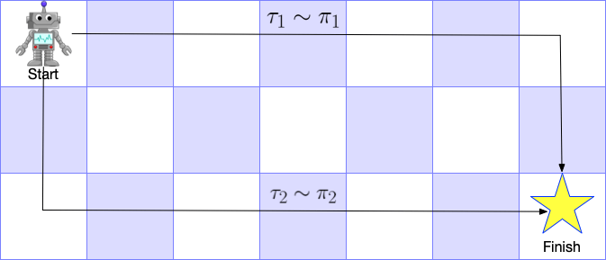
In this example, the task for the robot is to navigate to the star (right bottom corner) starting from the top left corner. Mathematically, we could model the process as an MDP described by a 6-tuple $(S,A,R,T,\gamma ,{\rho }_0)$.

• $S$ represents the state space. In our example, a state $s\in S$ could be which grid the agent is standing on.
• $A$ represents the action space. In the example, an action $a\in A$ could be trying to move to one of the four adjacent grid.
• $\gamma \in (0,1)$ is the temporal discount factor, representing the relative preference towards instant reward versus long-term reward.
• $R(s,a)$ represents the reward after executing action $a$ in the state $s$. In some cases, $R(s,a)$ could be simplified as $R(s)$. In our example, $R(s)$ is $0$ everywhere except for $+1$ for the star position.
• $T(s,a,s^{\prime })$ is the transition probability to $s^{\prime }$ from state $s$ after taking action $a$. For example, for the initial state and action “go right”, the agent will move one step right with probability $1$ if the robot is prefect. But if the robot is imperfect (which is always the case!), it is possible that the robot will instead go down with a probability $0.1$.
• ${\rho }_0(s)$ is the initial state distribution. In the example case, ${\rho }_0(s)$ has probability $1$ to be in the top left corner.

The standard goal of reinforcement learning is to find the optimal policy ${\pi }^{\ast }(a|s)$ that maximizes the discounted future reward, shown in Equation $\text{1}$.
$$\begin{array}{}\text{(1)}& J(\pi )={\mathbb{E}}_{\tau \sim \pi }\left[\sum _{i=0}^T{\gamma }^{t}R(s_t,a_t)\right]\end{array}$$
$\tau =(s_0,a_0,\cdots ,s_T,a_T)$ denotes a sequence of states and actions induced by the policy and dynamics: $s_1\sim {\rho }_0(s)$, $a_t\sim \pi (\cdot |s_t)$, $s_{t+1}\sim T(s_t,a_t,\cdot )$, $t\in \{1,2,\cdots ,T\}$.

We instead consider a more general maximum entropy objective which augments the standard objective with an entropy bonus to favor stochastic policies and to encourage exploration during optimization by [Zierbart 2008], shown in Equation $\text{2}$.
$$\begin{array}{}\text{(2)}& J(\pi )={\mathbb{E}}_{\tau \sim \pi }[\sum _{i=0}^T{\gamma }^{t}R(s_t,a_t)+\alpha H(\pi (\cdot |s_t))]\end{array}$$

What is Inverse Reinforcement Learning?

Inverse Reinforcement Learning (IRL) considers an MDP sans reward function ($M\mathrm{\setminus }R$) with the goal being to infer reward function $R(s,a)$ given a set of demonstrated trajectories $\mathcal{D}=\{{\tau }_1,{\tau }_2,\cdots ,{\tau }_N\}$. For example, in Figure 1, we draw two demonstrated trajectories ${\tau }_1$ and ${\tau }_2$. A typical assumption for IRL is that demonstrated trajectories are optimal, or at least near-optimal or stochastic optimal. In the case of our example ($R(s)$ is $0$ everywhere except for $+1$ for the star position), both trajectories are optimal, i.e., obtaining the $+1$ reward with the least time.

Adversarial Inverse Inforcement Learning (AIRL) casts the problem of LfD in a generative adversarial framework, learning a discriminator, $D$, to distinguishes between experts and a deceiving generator, $\pi$, that learns to imitate the expert. This framework follows Maximum-Entropy IRL’s assumption that trajectory likelihood is proportional to the exponential of trajectory rewards, i.e. $p(\tau )\propto \sum _{t=1}^T{\gamma }^t{r}_t$. The Discriminator $D$ is defined in Equation $\text{3}$, where $f_{\theta }(\tau )$ is the learnable reward function and $\pi$ is the current policy. $D$ is updated by minimizing its cross entropy loss to distinguish expert trajectories from generator policy rollouts (Equation $\text{4}$). Generator $\pi$ is trained via RL (Equation $\text{2}$) to maximize the pseudo-reward function given by $f(s,a)$.
$$\begin{array}{}\text{(3)}& D_{\theta }(s,a)=\frac{\exp (f_{\theta }(s,a))}{\exp (f_{\theta }(s,a))+\pi (a|s)}\end{array}$$

$$\begin{array}{}\text{(4)}& L_D=-{\mathbb{E}}_{\tau \sim \mathcal{D},(s,a)\sim \tau }[& \log D(s,a)]-{\mathbb{E}}_{\tau \sim \pi ,(s,a)\sim \tau }[1-\log D(s,a)]\end{array}$$

TL;DR: IRL algorithms (including AIRL) learn a reward function that could explain demonstration behavior. Further, IRL trains a policy that maximizes the learned reward, which should behave similarly to the demonstration.

Multi-Strategy Reward Distillation Method

In MSRD, we consider heterogeneous demonstration dataset, ${\mathcal{D}}^{(i)}=\{{\tau }_1^{(i)},{\tau }_2^{(i)},\cdots ,{\tau }_M^{(i)}\}$, where $i\in \{1,2,\cdots ,N\}$ is strategy index, $M$ is the number of demonstration trajectories for one strategy, and $N$ is the number of strategies. In our robot navigation example, ${\mathcal{D}}^{(1)}=\{{\tau }_1^{(1)}\},{\mathcal{D}}^{(2)}=\{{\tau }_1^{(2)}\}$, i.e., there are two different strategies, and each strategy has one demonstration.

The core assumption of MSRD is fairly straightforward: the reward function in each demonstration is optimizing is a linear combination of the task reward ($R^{(0)}$) and the strategy-only reward as given by Equation $\text{5}$. We call ${\tilde{R}}^{(i)}$ strategy-only reward. When strategy-only reward is combined with task reward, it becomes strategy-combined reward ($R^{(i)}$), meaning one wants to finish the task as well as maintaining the strategy.
$$\begin{array}{}\text{(5)}& R^{(i)}(\cdot )& =R^{(0)}(\cdot )+{\alpha }_i{\tilde{R}}^{(i)}(\cdot )\end{array}$$

Our approach is unique in that it shares the task reward with all the demonstrations while having the ability to tease out demonstrator-specific nuances (i.e., heterogeneity).

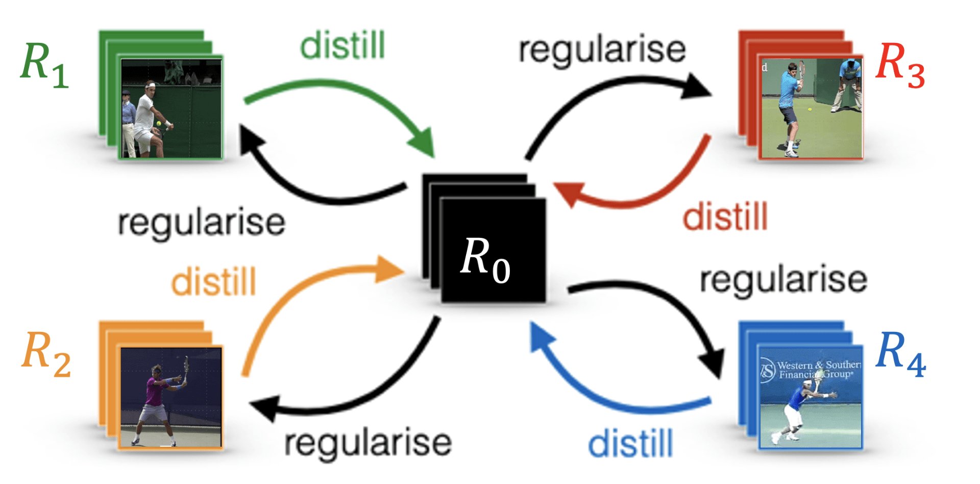
To infer the shared task reward function, we propose utilizing network distillation to distill common knowledge from each separately learned strategy-combined reward $R^{(i)}$ to the task reward function $R^{(0)}$. The learning diagram is shown in Figure 2. We also want to regularize $R^{(i)}$ to be close to $R^{(0)}$, since we have the prior knowledge that despite heterogeneous strategic preferences, all experts should still be prioritizing optimizing the task reward $R^{(0)}$ to achieve at least near-optimal performance. We propose to regularize the expected L2-norm of the difference between the reward functions, as shown in Equation $\text{6}$, in which ${\pi }^{(i)}$ is the optimal policy under reward function $R_{{\theta }_i}^{(i)}$.
$$\begin{array}{}\text{(6)}& L_{\text{reg}}={\mathbb{E}}_{(s,a)\sim {\pi }^{(i)}}\left({\left||R_{{\theta }_i}^{(i)}(s,a)-R_{{\theta }_0}^{(0)}(s,a)|\right|}_2\right)\end{array}$$
Note that we are using an index both on $\theta$ and $R$ to denote that each strategy-combined reward $R^{(i)}$ has its own reward parameters, and that these are approximated by separate neural networks with parameters ${\theta }_i$ for each strategy and ${\theta }_0$ for the task reward. There is no parameter sharing between strategy and task reward.

To avoid computational cost to fully optimize ${\pi }^{(i)}$ and $R^{(i)}$, we apply an iterative reward function and policy training schedule similar to AIRL. Combining AIRL’s objective (Equation $\text{4}$) with the distillation objective, we want to maximize $L_D$ in Equation $\text{7}$.
$$\begin{array}{}\text{(7)}& L_D=\sum _{i=1}^N& [{\mathbb{E}}_{(s,a)\sim {\tau }_j^{(i)}\sim {\mathcal{D}}^{(i)}}\log D_{{\theta }_i}(s,a)+{\mathbb{E}}_{(s,a)\sim {\pi }^{(i)}}\log (1-D_{{\theta }_i}(s,a))–{\mathbb{E}}_{(s,a)}\left({\left||R_{{\theta }_i}^{(i)}(s,a)-R_{{\theta }_0}^{(0)}(s,a)|\right|}_2\right)]\end{array}$$
Yet, while Equation $\text{7}$ should be able to distill the shared reward into $R_{{\theta }_0}^{(0)}$, the distillation is inefficient as $R_{{\theta }_0}^{(0)}$ will work as a strong regularization for $R_{{\theta }_i}^{(i)}$ before successful distillation.

Instead, our structure in Equation $\text{5}$ allows for a two-column (reference) re-parameterization, speeding up knowledge transfer and making the learning process easier. Combining Equation $\text{5}$ and Equation $\text{7}$, we arrive at Equation $\text{8}$.

$$\begin{array}{}\text{(8)}& L_D& =\sum _{i=1}^N[{\mathbb{E}}_{(s,a)\sim {\tau }_j^{(i)}\sim {\mathcal{D}}^{(i)}}\log D_{{\theta }_i,{\theta }_0}(s,a)+{\mathbb{E}}_{(s,a)\sim {\pi }^{(i)}}\log (1-D_{{\theta }_i,{\theta }_0}(s,a))–{\alpha }_i{\mathbb{E}}_{(s,a)}\left({\left||{\tilde{R}}_{{\theta }_i}^{(i)}(s,a)|\right|}_2\right)]\end{array}$$

The key difference between Equation $\text{8}$ and Equation $\text{7}$ is that $D$ depends on both $R_{{\theta }_0}^{(0)}$ and ${\tilde{R}}_{{\theta }_i}^{(i)}$ instead of separate $R_{{\theta }_i}^{(i)}$. Thus, $R_{{\theta }_0}^{(0)}$ directly updates from the discriminator’s loss rather than waiting for knowledge to be learned by a strategy-combined reward and subsequently distilled into a task reward.

Further, the last term of Equation $\text{8}$ reduces to a simple L2-regularization on strategy-only reward’s output, weighted by ${\alpha }_i$. This formulation provides us with a new view to interpret the relative weights of the strategy-only reward ${\alpha }_i$: the larger ${\alpha }_i$ is, the more the strategy-only reward will influence the strategy-combined reward. Therefore, we will have higher regularization to account for possible overwhelming of the task reward function. Comparing Equation $\text{8}$ and $\text{4}$, we could interpret MSRD in another view: optimizing ${\theta }_i$ only via IRL objective results in a combination of task and strategy reward, and adding regularization on the strategy reward will encourage to encode only necessary information in ${\theta }_i$ and share more knowledge in ${\theta }_0$.

Simulation Results

We tested MSRD on two simulated environments: inverted pendulum and hopper. The goal of the inverted pendulum task is to balance a pendulum on a cart by moving the cart left/right. The reward for the inverted pendulum is defined as the negative absolute value of the pendulum angle from the upright position. The objective of hopper is to control 3-DoF joints to move forward. The reward for hopper is defined as the speed at which it moves forward. We removed termination judgments to gain flexibility in behaviors.

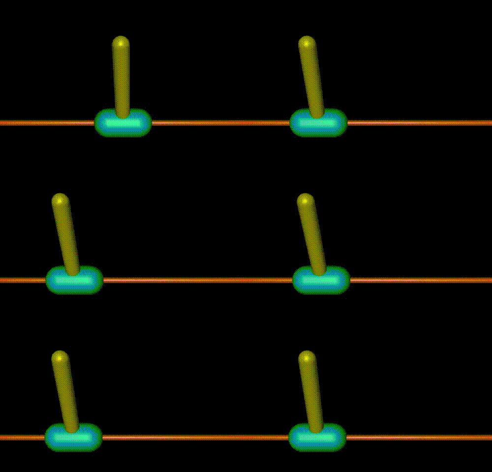
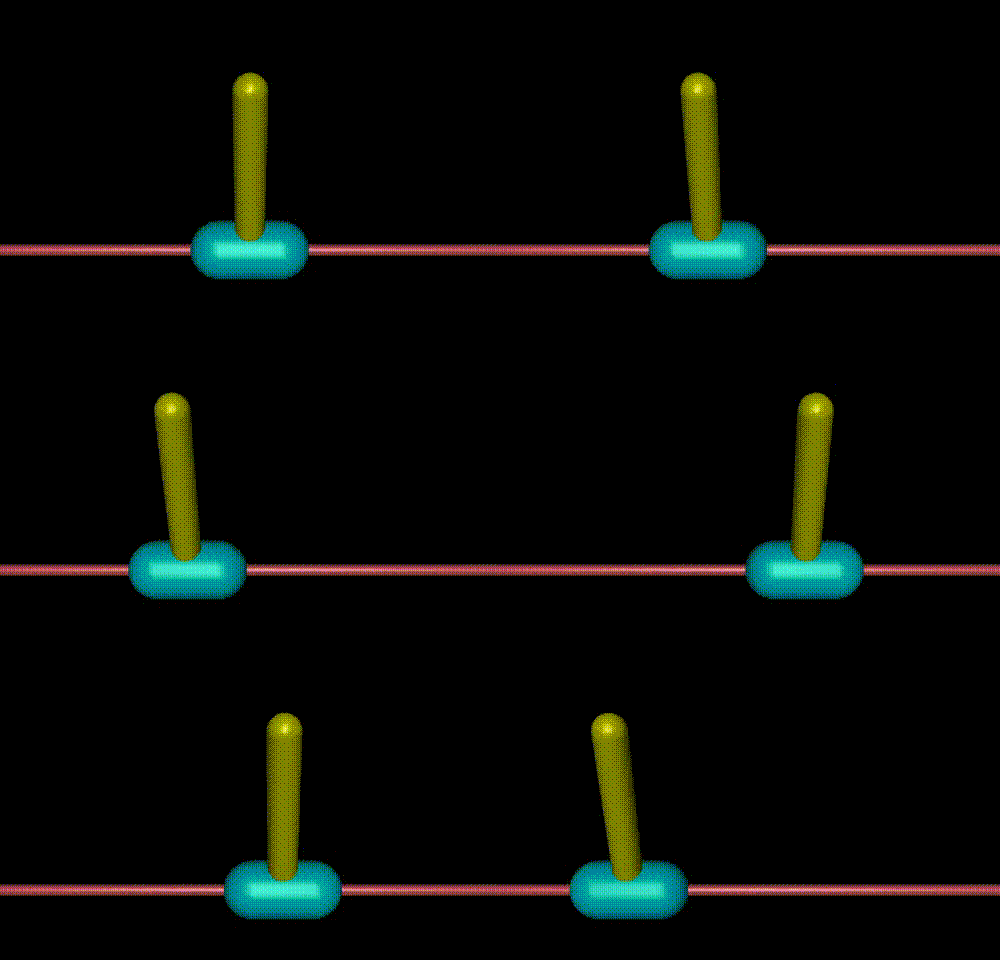
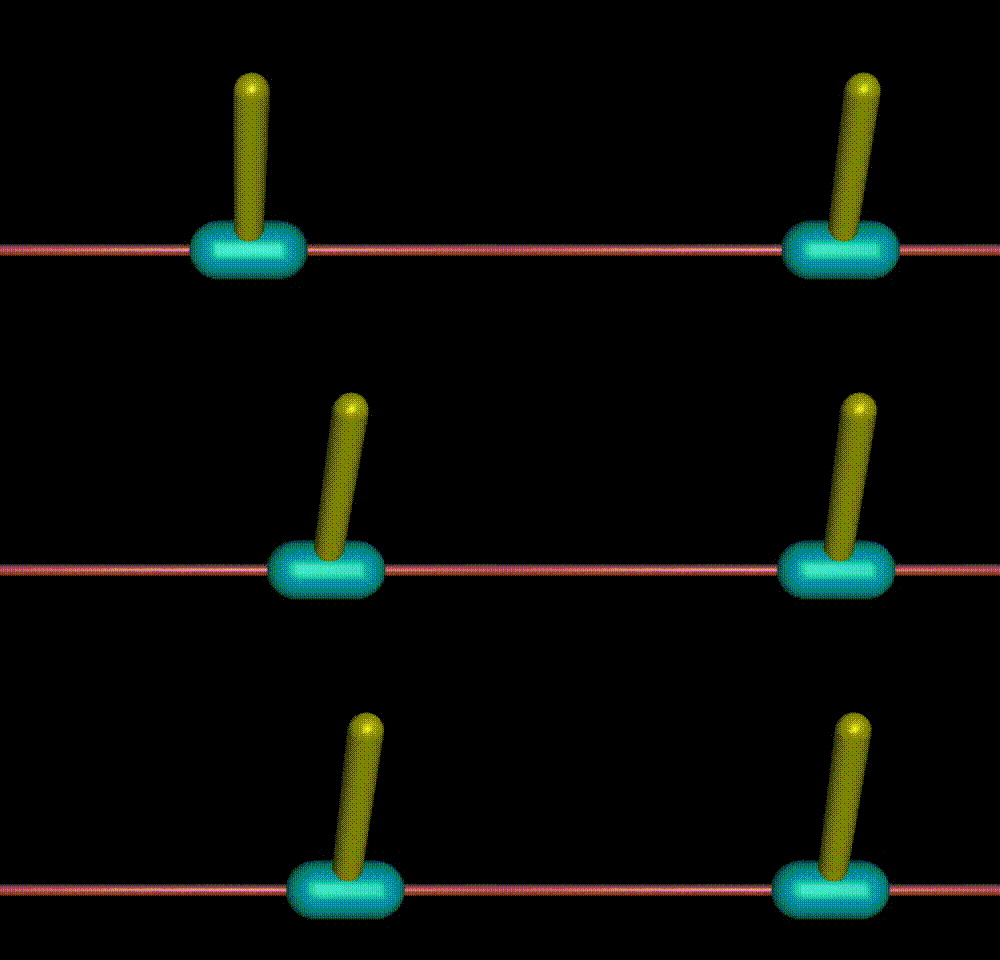
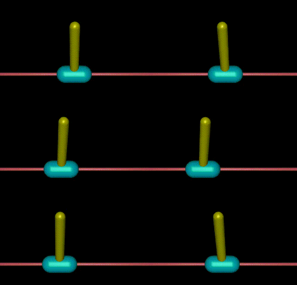
We first generated a variety of demonstrations to emulate heterogeneous strategies that humans will apply in solving problems for our virtual experiments via “DIAYN + Extrinsic Reward” and a novel method called “KL-Encouraged + Extrinsic Reward”. The two methods essentially encourage the policies trained to be different from each other while still accomplishing the task goal. We generated 20 different strategies for Inverted Pendulum and 2 most significant strategies for hopper, shown in Figure 3 and Figure 4.

Hypotheses

We explore two hypotheses to elucidate MSRD’s advantage on recovering both the latent task reward (the essential goal of the demonstrators) and the means by which the task is accomplished (i.e., the strategy):

H1: The task reward learned by MSRD has a higher correlation with the true task reward than AIRL.
H2: Strategy-only reward learned by MSRD has a higher correlation with true strategic preferences than AIRL.

We assessed both hypotheses quantitatively and qualitatively for the simulation environments as the ground-truth reward functions are available.

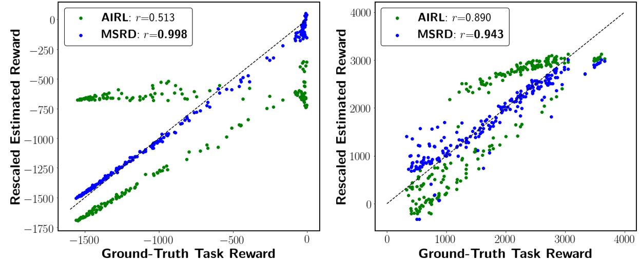
To test H1, we constructed a dataset of trajectories that have various task performances. We then evaluated the reward function learned by AIRL and MSRD on the trajectories, comparing estimated vs. ground-truth rewards. We show a correlation of estimated rewards and ground-truth task rewards in Figure 5. The task reward function learned through MSRD has a higher correlation with the ground-truth reward function (0.99 and 0.94) versus AIRL (0.51 and 0.89) for each domain, respectively. AIRL’s reward function overfits to some strategies and mixes the task reward with that strategy-only reward, making its estimation unreliable for other strategies’ trajectories.

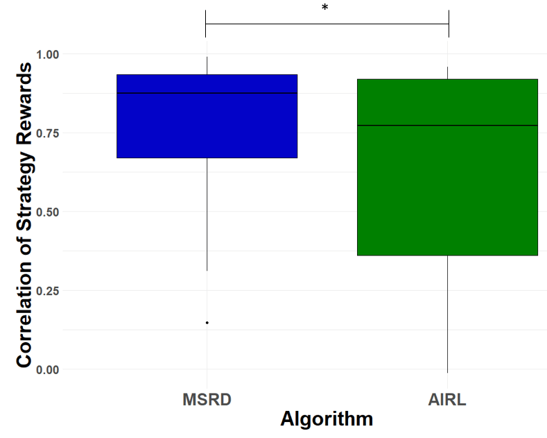
To test H2, we calculated the correlations of MSRD’s strategy-only rewards with the true strategic preferences and compared that with the correlation of AIRL’s rewards when AIRL is trained on each individual strategy. In simulated domains, true strategic preferences are available. Correlations of both methods for all strategy rewards in inverted pendulum are shown in Figure 6. A paired t-test shows that MSRD achieves a statistically significantly higher correlation (M = 0.779, SD = 0.239) for the strategy rewards versus AIRL (M = 0.635, SD = 0.324) trained separately for each strategy, $t(19)=1.813$, $p=0.0428$ (one-tailed). A Shapiro-Wilk test showed the residuals were normally distributed ($p=0.877$). For the hopper domain, MSRD achieved $0.85$ and $0.93$ correlation coefficient for the hop and crawl strategy, compared with AIRL’s $0.80$ and $0.82$ respectively.

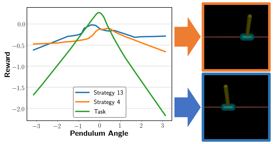
We further show qualitative results for the learned strategy reward. For Inverted Pendulum, we fix three dimensions (cart position, cart velocity and pendulum angular velocity) to zero and investigate the reward change within the one remaining dimension (pendulum angle). The relationship between rewards and pendulum angles in task and strategy reward functions are illustrated in Figure 7, in which the task reward function reaches its peak when the angle of the pendulum is near zero. This precisely recovers the task reward. For strategy-only reward functions, strategy 13 encourages the pendulum to lean left, while strategy 4 encourages the policy to tilt the pendulum right. Therefore, strategy-only rewards learned by MSRD captures specific preferences within demonstrations. Figure 7 also shows the magnitude of the task reward is larger than the strategy reward, which affirms our expectation that an emphasis is being put towards accomplishing the task.

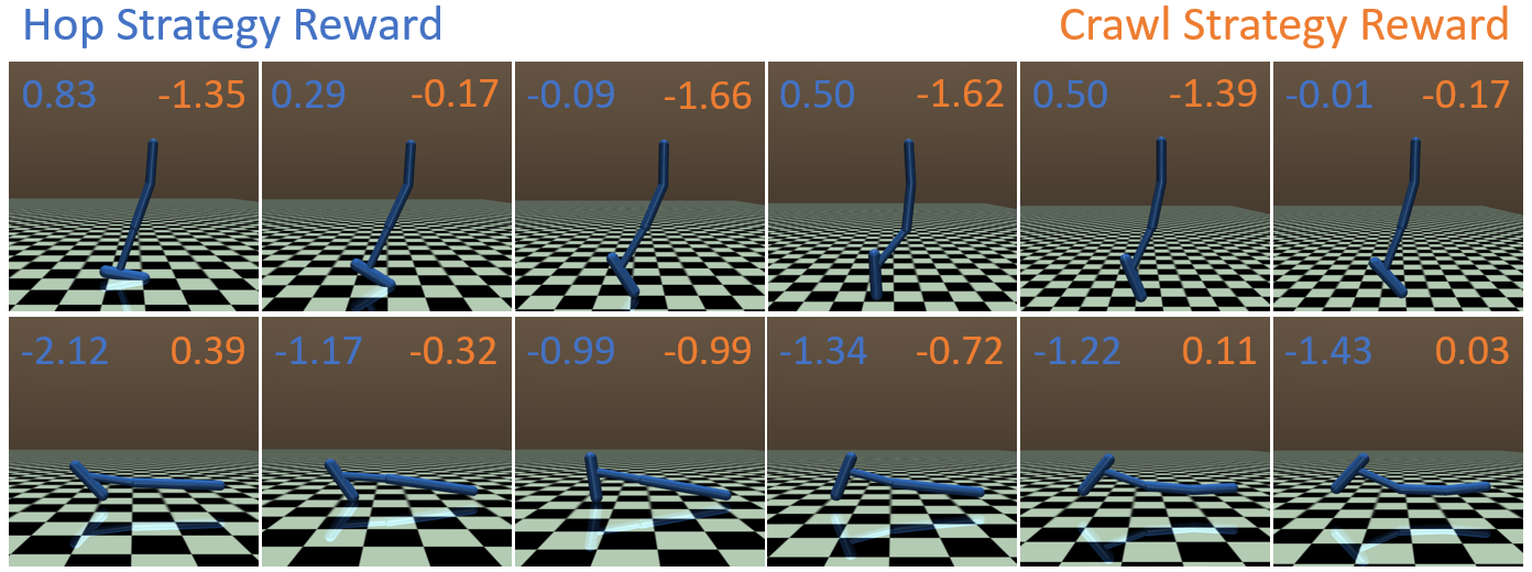
In the hopper environment, it is harder to visualize the reward landscape due to a high-dimensional observation space and a lack of interpretability of states. Therefore, instead of visualizing a reward curve, we evaluate the estimated strategy-only reward on trajectories from both strategies. Figure 8 shows that when given a hopping trajectory, the hop strategy-only reward function gives higher reward for that behavior than crawl strategy-only reward function. Similarly, in the crawl trajectory case, the crawling strategy-only reward gives a higher value than the hop strategy-only reward. Therefore, the strategy-only reward function recovered by MSRD gives a higher reward to the corresponding behavior than the other strategy-only reward function, thus providing encouragement to the policy towards the intended behavior.

These results across our simulated environments show our algorithms’ success in both task reward recovery and strategy reward decomposition. This capability is a novel contribution to the field of LfD in that we are able to tease out strategies from the underlying task and effectively learn policies that can reproduce both the strategy and a well-performed policy for the underlying task.

Robot Table Tennis Results

We tested MSRD on its capability to learn various table tennis strokes from expert human demonstration. Participants were asked to kinetically teach a robot arm to hit an incoming ping pong ball using three different stroke strategies: push, slice, and topspin. The change in angle and the upward/downward motion of the paddle throughout the policy trajectory are key factors in the display of different strategies (as these induce spin). Push is associated with a small change in angle as it is not attempting to add any spin onto the ball. Slice places a backspin on the ball, and thus the angle of the paddle will quickly tilt up. Conversely, to achieve a topspin on the ball, the associated trajectory has a quick upward motion.

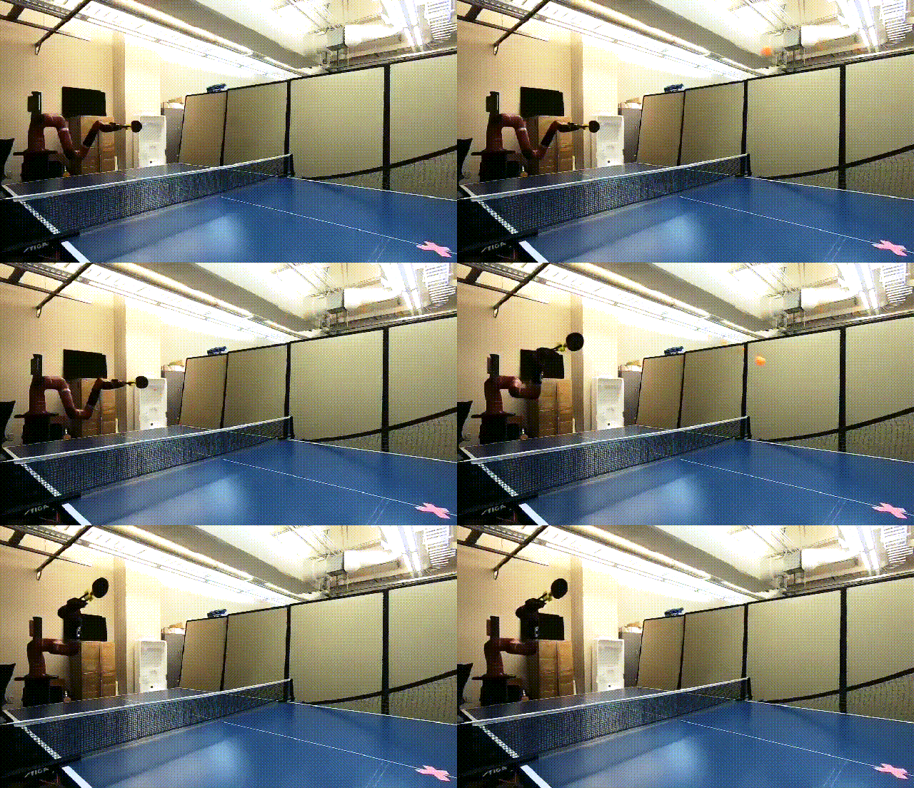
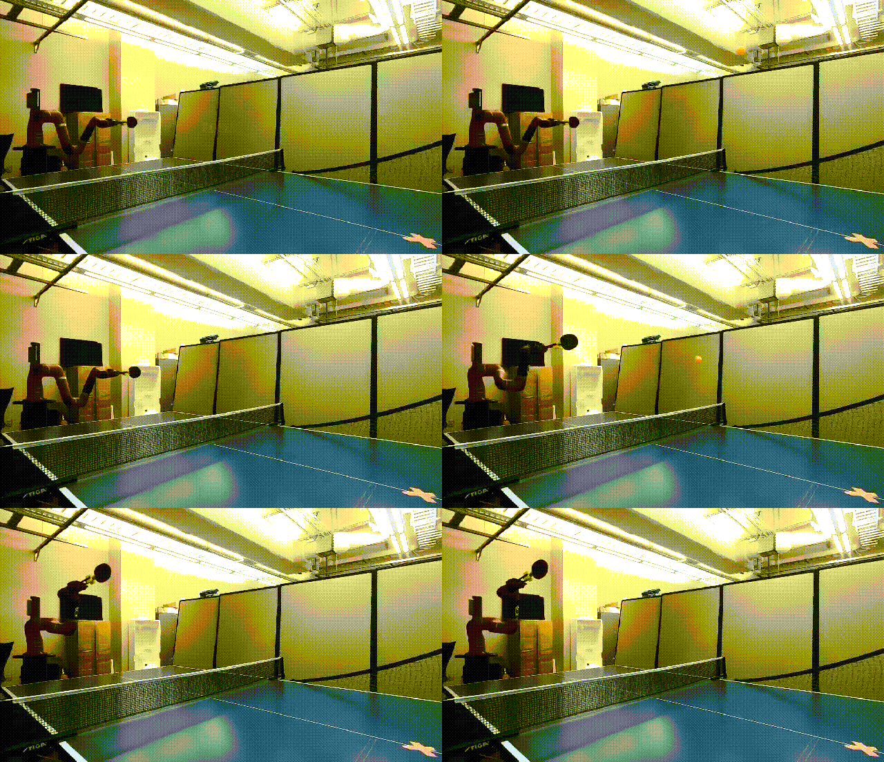
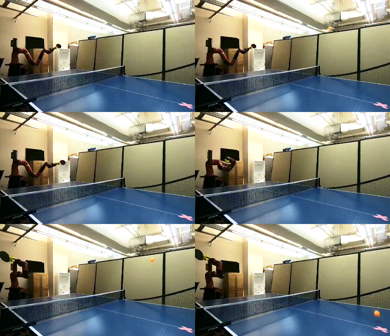
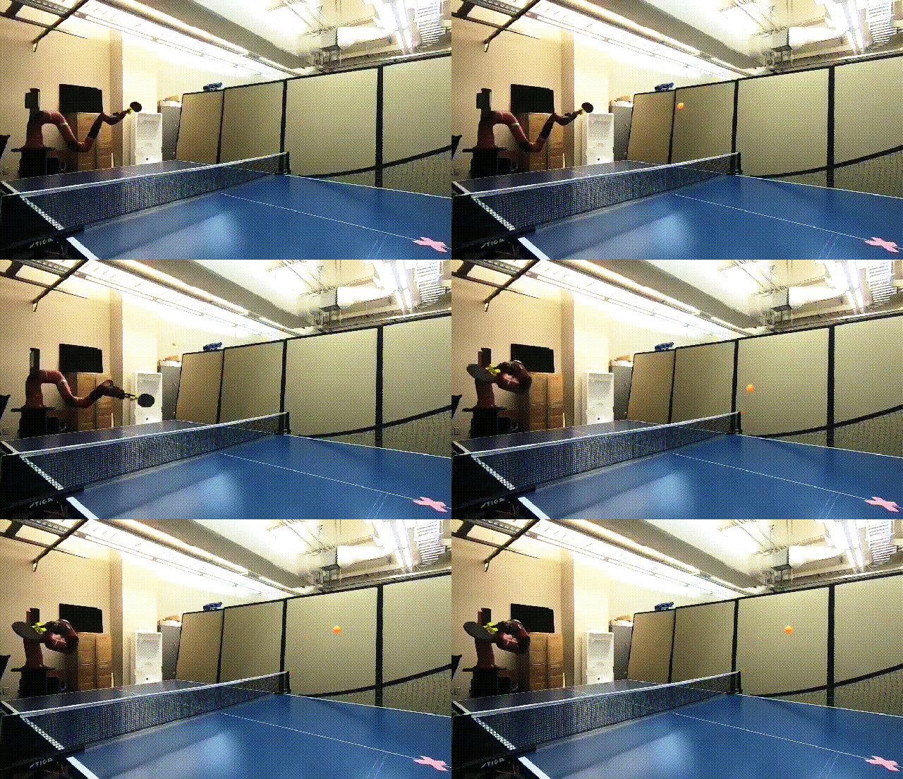
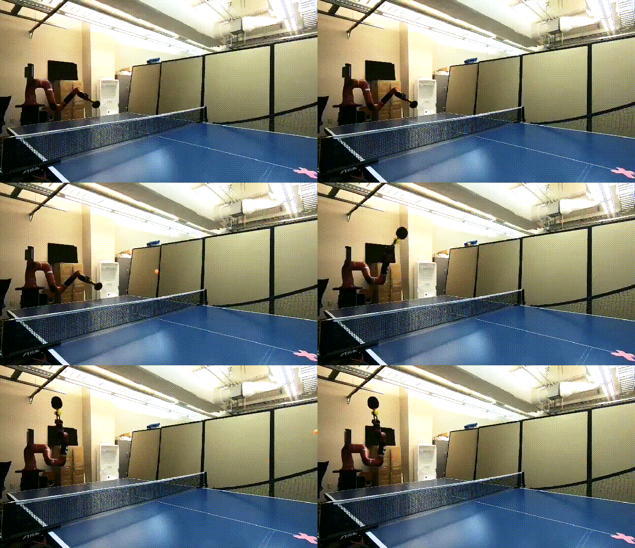
After just 30 minutes of training on each strategy, the robot was able to learn to strike $83\mathrm{\%}$ of the fed balls, shown in Figure 9. The robot learned to perform all strategies, and the robot’s best strategy, topspin, resulted in $90\mathrm{\%}$ of balls returned successfully.

Conclusion

We explored the important case of IRL when demonstrators provide heterogeneous, strategy-based demonstrations besides seeking to maximize a latent task reward. By explicitly modeling the task and strategy reward separately, and jointly learning both, our algorithm is able to recover more robust task rewards, discover unique strategy rewards, and imitate strategy-specific behaviors.