1. Motivation

Given the recent developments in robotic technologies and the increasing availability of collaborative robots (cobots), multi-robot systems are increasingly being adopted in various environments, including manufacturing, warehouse, and hospitals. Research in related areas (e.g., multi-robot communication, team formation and control, path planning, task scheduling and routing) has also received significant attention. Our research focuses on multi-robot task allocation and scheduling. As an example, consider coordinating a team of robots to construct automotive parts, where different tasks are required at different workstations and have various time requirements to be satisfied (e.g., a certain amount of waiting time is needed between painting tasks to let the previous coat of paint fully dry). The goal is to try to find an optimal schedule, detailing which robot each task is assigned to and in which order the tasks are processed by each robot, while maximizing/minimizing a user-specified objective (e.g., total time used, total resource consumption).

Conventional approaches to multi-robot scheduling involve formulating the problem as a mathematical program and leveraging commercial solvers or developing custom-made approximate and meta-heuristic techniques. However, multi-robot scheduling with both temporal and spatial constraints is generally NP-hard. This means that exact methods always fail to scale to large-scale problems, which is exacerbated by the need for near real-time solutions to prevent factory slowdowns. Alternatively, heuristic approaches are lightweight and effective. Yet, designing good heuristics involves a combined, herculean effort from computer scientists, operations researchers, and industrial engineers that leaves much to be desired. Moreover, the performance of heuristics is usually bound with specific objective functions. Even with the same kind of problems, when the optimization objective changes, new efforts are needed to re-design the heuristics to perform well again.

In recent years, deep neural networks have brought about breakthroughs in many domains, including image classification, nature language understanding and drug discovery, as neural nets can discover intricate structures in high-dimensional data without hand-crafted feature engineering. Can deep learning save us from the tedious work of designing application-specific scheduling solutions? It will be desirable to let the computer to autonomously learning scheduling policies without the need of domain experts. Promising progress has been made towards learning heuristics for combinatorial optimization problems. Yet previous research focuses on significantly easier problems than the multi-robot scheduling problem. To push this idea further, we try to develop a novel neural networks-based model that learns to reason through the complex constraints in multi-robot scheduling for constructing high-quality solutions.

2. Problem Details

To evaluate the idea of using deep learning for scheduling solution development, we look into a popular application domain of robot teams: final assembly manufacturing. To begin with, based on difficulties encountered in such scenario, we extract the problem as coordinating a multi-robot team in the same space, with both temporal and resource/location constraints.

Specifically, a problem instance consists of the following components:

1. A team of robots that are assumed to be homogeneous in task completion.
2. A set of tasks that each takes some time to complete. Here we consider two types of temporal constraints: a) deadline constraints specifying that a task has to be completed before a certain time point; 2) wait constraints specifying the relative wait time between two tasks.
3. A set of locations. At most, one task can be performed at each location at the same time.
4. And an objective function to minimize. A common choice is the total makespan (i.e., overall process duration) and is used in the evaluation section.

A feasible solution to the problem consists of an assignment of tasks to robots and a time schedule for each robot’s tasks such that all constraints are satisfied. An optimal solution is the feasible solution that has the minimium objective value.

We want to learn a deep learning-based policy that can construct high-quality schedules for given problem instances. The first thing is to formulate scheduling as a sequential decision-making problem, in which individual robots’ schedules are collectively, sequentially constructed in a rollout fashion. At each decision step, the policy picks a robot-unscheduled task pair and assigns the selected task to the end of the selected robot’s schedule. This step repeats until all tasks are scheduled. As a result, we can formalize schedule generation as a Markov Decision Process (MDP) that includes:

1. A problem state includes the description of the problem, with time constraints, resource constraints, and all robots’ partial schedules constructed so far.
2. An action takes the form of an (unscheduled task, robot) pair that corresponds to appending the selected task to the end of the partial schedule of the selected robot.
3. The transition of states corresponds to updating the partial schedule of the selected robot.
4. The immediate reward of a state-action pair is defined as the change in makespan of all the scheduled tasks after taking the action. As such, the cumulative reward of the whole schedule generation process equals the final makespan of the problem (when feasible solutions are found).
5. A discount factor.

We aim to learn a policy that schedules tasks and agents following the MDP. A common way in policy learning is to learn a value function parameterized by neural networks. In our case, our goal is to approximate the Q value (future discounted total reward) function with a neural network $\hat{Q}_\theta$ parameterized by weights $\theta$. Then, we obtain a greedy policy $\pi := \mathrm{argmax}_u \hat{Q}_\theta$ that selects a task and a robot at each step to maximize the Q value with corresponding action $u$.

However, because the problem state includes temporal constraints that are represented by inequalities, it is not straight forward to learn high-level embeddings from them. Fortunately, there is an alternative way of representing those temporal constraints: using simple temporal networks (STNs). This makes it possible to utilize graph neural networks (GNNs) for parameterizing the problem states and actions for Q value prediction, by directly operating GNNs on STNs.

3. STN meets GAT

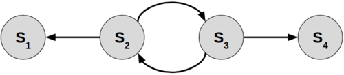
A simple temporal network (STN) is the graph representation of a Simple Temporal Problem (STP). An STN is a directed edge-weighted graph <$V$, $E$> where $V$ is the set of nodes and $E$ the set of edges. Each node represents an event-related time point. Each edge, $i$ -> $j$, is labeled by a weight $a_{ij}$, representing the linear inequality $X_j-X_i \leq a_{ij}$.

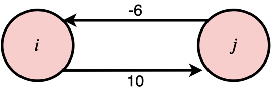
Fig. 1 A simple temporal network

Figure 1 displays an STN with two nodes and two edges. It is easy to see that the two edges impose the following constraints.

\begin{equation}
6 \leq X_j – X_i \leq 10
\end{equation}

So what does it look like when using it to represent our problem instances? Figure 2 is an example STN involving 3 tasks, where each task is associated with a start time node $s_i$ and an end time node $f_i$.

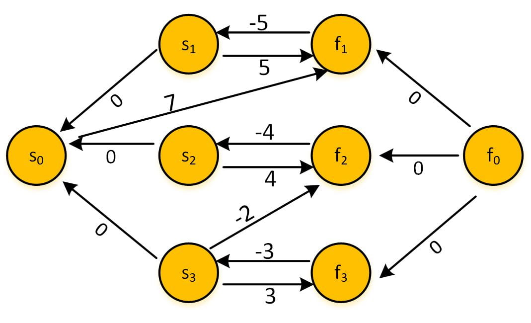
Fig. 2 An STN with start and finish nodes for three tasks, as well as placeholder start and finish nodes, $s_0$ and $f_0$

From the edge $s_0$->$f_1$: 7, we can get $f_1 – s_0 \leq 7$, which is just $f_1 \leq 7$, imposing a deadline constraint for task 1. There is also a wait constraint between task 2 and 3: from $s_3$->$f_2$: -2, we have: $f_2 – s_3 \leq -2$, which means $s_3 \geq f_2 + 2$.

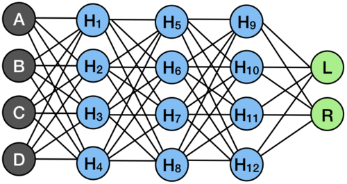
Then our challenge boils down to developing a GNN model that operates on the STN structure to learn embeddings of each node (time event). Analogous to the convolutional neural networks (CNNs) for feature-learning in images, GNNs can hierarchically learn high-level representations of graph structures through graph convolutions and backpropagation. Modern GNNs capture the dependence of graphs via message-passing between the nodes, in which each node aggregates feature vectors of its neighbors from previous layers to compute its new feature vector. After $k$ layers of aggregation, a node $v$’s representation captures the structural information within the nodes that are reachable from $v$ in $k$ hops or fewer. Systems based on GNNs have demonstrated ground-breaking performance on tasks such as node classification, link prediction, and clustering. We make use of the graph attention layer (GAT) proposed in this ICLR 2018 paper, which introduces an attention mechanism to graph convolutional layers to improve generalizability.

While the original GAT layer deals with undirected, unweighted graphs, STNs are directed weighted graphs where temporal constraints are represented by the direction and attribute of the edge. These differences lead to two adaptations.

1. The message passing follows the same direction of the edge, which means that we only consider the incoming neighbors when aggregating node features.
2. We incorporate the edge attribute into both the feature update phase and attention coefficient calculation phase.

As a result, the forward pass of our adapted graph attention layer can be illustrated in figure 3.

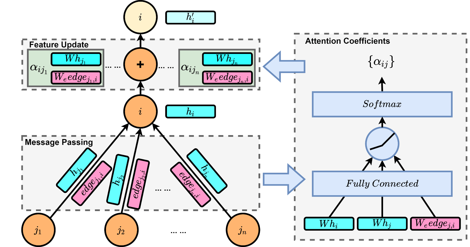
Fig. 3 The forward pass of the adapted graph attention layer (left-hand side), which consists of two phases: 1) Message passing: each node receives features of its neighbor nodes and the corresponding edge weights; 2) Feature update: neighbor features are aggregated using attention coefficients; the right-hand side illustrates how attention coefficients are calculated.

It is not hard to derive the update equations for each node as following.

\begin{equation}
\vec h_i^\prime = \mathrm{ReLU} \Big (\sum_{j \in N(i)} \alpha_{ij} (W \vec h_j+W_e edge_{ji}) \Big )\label{eq:GAT_layer}
\end{equation}

\begin{equation}
\alpha_{ij} = \mathrm{softmax}_j \bigg( \sigma \left(\vec a^T\left[W \vec h_i || W \vec h_j || W_e edge_{ji}\right]\right) \bigg) \label{eq:attention}
\end{equation}

Here $N(i)$ is the set of neighbors of node $i$, $W$ is the weight matrix applied to every node, $\vec h_j$ is the node feature from the previous layer, and $\alpha_{ij}$ are the attention coefficients. For calculating attention coefficients, $\vec a$ is the learnable weight, $||$ represents concatenation, and $\sigma()$ is the LeakyReLU nonlinearity. Softmax function is used to normalize the coefficients across all choices of $j$.

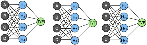
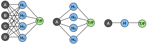
Now that we have a GAT layer that operates on the STN, the next step is to define robot-specific node features to calculate the embeddings of each robot given a problem STN updated with partial schedules. “Robot-specific” means that the node features are generated with respect to a particular robot. Those features include binary encoding denoting whether the corresponding task is scheduled to this robot, to other robots, or not scheduled. The input features also consist of task location information which is not present in the STN. Given an STN and a set of robot-specific node features, the graph attention network, constructed by stacking several GAT layers, outputs the embeddings of each node w.r.t. different robots. The embedding of the corresponding robot is obtained by averaging over all node embeddings of that robot. The state embedding is approximated by averaging over all robot embeddings. The action embedding is approximated by the node embedding of related STN time nodes calculated with robot-specific node features w.r.t. the selected robot. After this, all we need is to stack several fully-connected layers on top of the state-action embeddings to estimate the Q value. By using robot-specific node features, the network is non-parametric in both the number of tasks and the number of robots.

4. Policy learning: Q-learning vs. Imitation

Under the MDP formulation and a Q function based on GNN, we first considered training the policy using reinforcement learning algorithms like deep Q-learning. However, reinforcement learning relies on finding feasible schedules to learn useful knowledge. In our problems, most permutations of the schedule are infeasible. We found that the training was not stable and plenty of time was wasted while exploring infeasible solutions before the policy could learn anything useful, which was very ineffective.

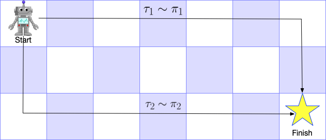
Instead, we turn to imitation learning methods that learn from high-quality schedules to accelerate the learning process for quick deployment. We belive in most cases it is practical to optimally solve small-scale scheduling problems with exact methods. Given the scalability of GNNs, we expect that exploiting such expert data on smaller problems to train the policy can generalize well towards solving unseen problems, even in a larger scale.

Let $D_{ex}$ denote the expert dataset that contains schedules either from exact solution methods or the domain experts. For each expert solution, we arrange the scheduled tasks by task start time in ascending order and decompose them into state-action pairs following our schedule generation process. This enables us to directly calculate the total reward of each state-action pair using $R_t^{(n)} = \sum_{k=0}^{n-t} \gamma^k R_{t+k}$ and regress the predicted Q values with a supervised loss $L_{ex}$.

\begin{equation}
L_{ex} = ||\hat{Q}_{\theta, expert}-R_t^{(n)}||^2
\end{equation}

To fully exploit the expert data, we ground the Q values of actions that are not selected by the expert to a value below $R_t^{(n)}$ using the loss shown below.

\begin{equation}
L_{alt} = \frac{1}{N_{alt}}\sum \left\lVert\hat{Q}_{\theta, alt}-\min(\hat{Q}_{\theta, alt}, R_t^{(n)} – q_o)\right\rVert^2
\end{equation}

$\hat{Q}_{\theta, alt}$ is the predicted Q value estimated with alternate actions not chosen by the expert, and is compared with a positive constant $q_o$ under $R_t^{(n)}$. Consequently, the gradient propagates through all the unselected actions that have Q predictions higher than $R_t^{(n)}-q_o$. The total loss is the sum of the two, plus a L2 regularization term on the network weights.

5. Experimental results

To evaluate the performance of our GNN-based model (we call it the RoboGNN scheduler), we used randomly-generated problems simulating final assembly manufacturing with a multi-robot teamm, e.g. construction of an airplane fuselage. We generated problems involving a team of robots (team size ranging from two to five) in different scales: small (16–20 tasks), medium (40–50 tasks) and large (80–100 tasks), with both temporal constraints and proximity/location constraints described in Section 2.

We benchmarked our trained GNN scheduler against the following methods.

1. Earliest Deadline First (EDF) – a ubiquitous heuristic algorithm that assigns the available task with the earliest deadline to the first available worker.
2. Tercio – the state-of-the-art scheduling algorithm for this problem domain. Tercio combines mathematical optimization for task allocation and analytical sequencing test for temporospatial feasibility.
3. Gurobi – a commercial optimization solver from Gurobi Optimization. Results from Gurobi v8.1 are the exact baseline. Gurobi is also used to generated expert schedules for training set.

The RoboGNN scheduler was trained on small problems and the same model was evaluated on all problem scales. We evaluated our model in terms of proportion of problems solved and compared it with other methods, as shown in Figure 4. We also reported mean and standard deviation of the computation time for different methods above corresponding bars, based upon the problems solved by each method. The results showed that the RoboGNN scheduler found considerably more feasible solutions than both EDF and Tercio, wiht > 10x faster speed than Gurobi.

Fig. 4 Proportion of problems solved for multi-robot scheduling: (left) small problems (16–20 tasks); (middle) medium problems (40–50 tasks); (right) large problems (80–100 tasks). Results are grouped in number of robots. Mean and standard deviation of computation times (in parenthesis) for each method is shown above each group’s bar.

Another metrics we used was average makespan. Calculating average makespans on each methods’ feasible solutions gave us a comparison of solution quality, as shown in Figure 5. Here the makespan was normalized to the one found by Gurobi.

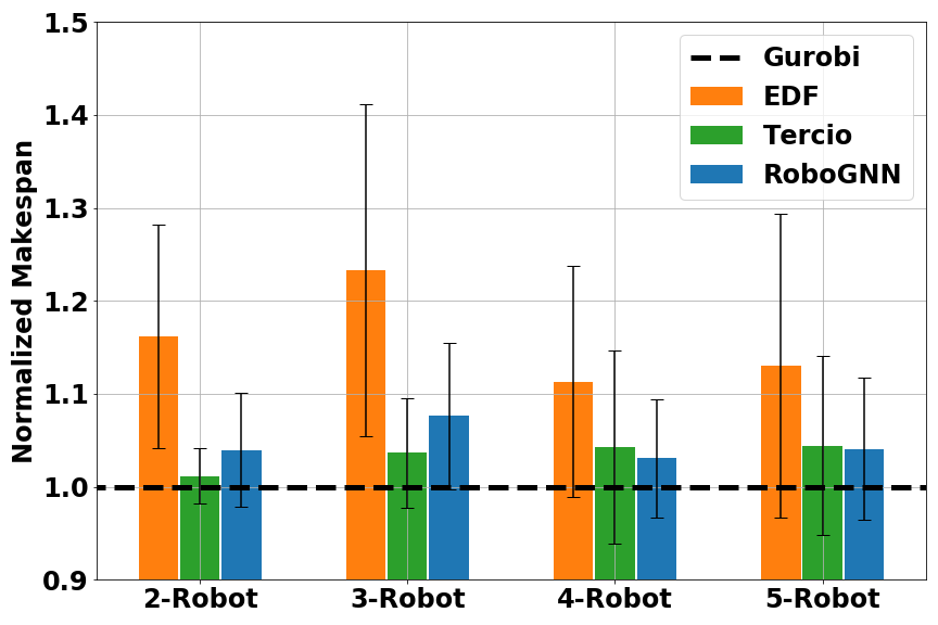
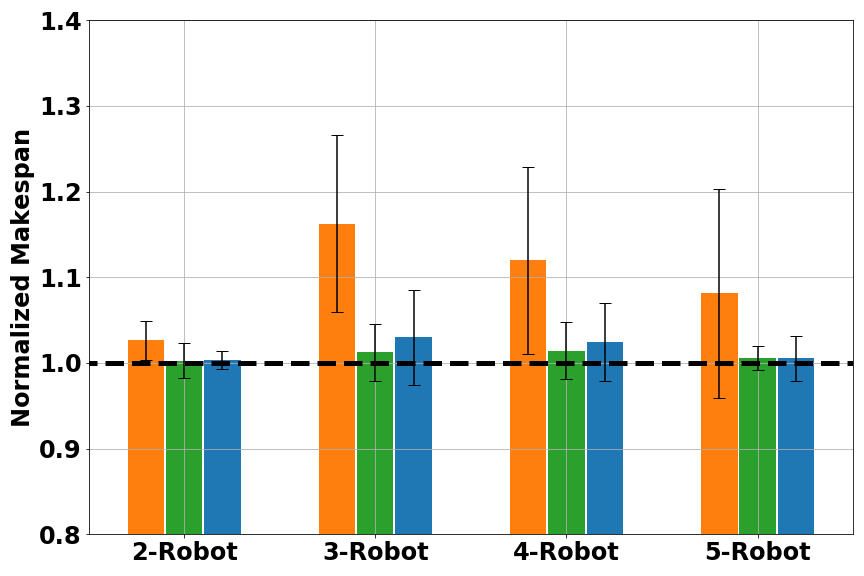
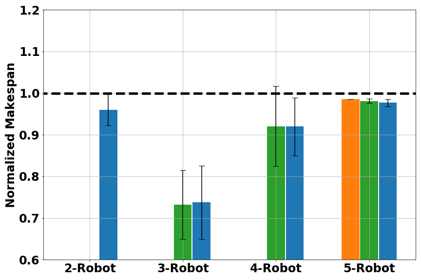
Fig. 5 Normalized makespan score for multi-robot scheduling: (left) small problems (16–20 tasks); (middle) medium problems (40–50 tasks); (right) large problems (80–100 tasks). Results are grouped in number of robots. A smaller (normalized) makespan is better.

Overall, RoboGNN and Tercio achieved similar makespan score, with EDF being the worst. For large problems, both RoboGNN and Tercio were able to find better solutions than Gurobi, with normalized makespan < 1. This was because we were comparing against the best solution Gurobi found with it a cutoff time of 1 hour, and optimally solving large scale problems with an exact method would cost much more time and computation resource than available. Considering that we only used expert data on small problems during training, the results provide strong evidence that our GNN-based framework is able to use knowledge learned on small problems to help solve larger problems.

6. Demo

So, how does the scheduling process look like? Thanks to the Robotarium, a remotely accessible swarm robotics research testbed with GRITSBot X robots, we are able to make a demo video.

This video demonstrates our trained RoboGNN scheduler to coordinate the work of a five-robot team in a simulated environment for airplane fuselage construction. The problem consists of eighteen tasks located randomly among 5 locations. The outputs of RoboGNN for action selection are shown as the schedule updates. For the first few choices, the GNN predictions are diverse among different tasks. For later choices, the predictions tends to be flat among the unscheduled tasks. This shows that to get a good schedule, it is crucial to correctly picking the beginning tasks.

Further Details

If you want to explore more on this, feel free to check our recent RA-L paper.

Acknowledgements

Thanks Esmaeil (Esi) Seraj and Dr. Matthew Gombolay for assistance with post editing and valuable feedback.

This entire post is a high-level summary of the motivations and contributions of my paper which was recently accepted to AISTATS 2020: Optimization Methods for Interpretable Differentiable Decision Trees in Reinforcement Learning.

Why aren’t normal neural networks interpretable?

Ultimately, neural networks are lots of matrix multiplication and non-linear functions in series. And following where a single number goes and how it affects the outcome of a set of matrix multiplication problems can be rather daunting.

Consider the cart pole problem from the OpenAI Gym. The objective of the challenge is to balance an inverted pendulum (the pole) on a cart that can shift left or right on a line. By just nudging gently left and right, it’s possible to keep the pole balanced upright. We can train agents to solve this problem without much issue, but if you wanted to visualize a network’s decision-making process, it wouldn’t be so easy. Then again, cart pole is a simple problem: There are only four variables in the state, and a network with two layers can solve the problem.

Perhaps the closest you could get is to draw out all of the different matrix multiplication operations that would need to take place, and then try to trace through the math each time. With such a simple problem and network, what might that look like?

As it turns out, it’s very complicated. To know what the network would do in any given state, we need to be able to run through 4 matrix multiplication problems, save the results, run through 2 more matrix multiplication problems, and then compare the two results you get. Even if we remove non-linear activations from the input-layer’s output, this is clearly not what we would conventionally call “interpretable.”

So what about differentiable decision trees?

Decision trees are a more classic machine learning approach which yield interpretability, simplicity, and ease of understanding. The actual format of a decision tree is essentially a list of “Yes or No” questions until the machine finally arrives at an answer.

Going back to cart-pole up above, we might say “If you’re to the left of center, move right. Otherwise, move left.” If we know that:

• “A” is the cart position,

• 0 is center, and

• negative is left,

then this is a very simple decision tree which could be drawn like so:

Now, this is a bit simplistic and in reality it wouldn’t actually do very well. There is a trade-off here between simplicity and performance. The complicated matrix math does quite well, but we can’t understand it. The dead-simple decision tree is very easy to understand, but it doesn’t do all that well. Can we combine the two?

As it turns out, yes! By structuring a network like a decision tree, we can learn how to perform well in a reinforcement learning environment, and then have all of the network’s “knowledge” captured in a convenient decision-tree shape. That doesn’t quite solve our matrix math problem, but it gets us closer.

Instead of a multi-layer network with obscure mappings and math, we have simpler single-layer checks which spit out a “True” or “False,” and eventually a very small pair of weights on different actions. Each check is itself a layer of the network, and the outputs are themselves sets of parameters. So instead of a multi-layer network like this:

We can sort of decompose our network into mini sub-networks, where each mini-network is a single decision in the tree.

While this isn’t much simpler, we got rid of a nasty set of repeating hidden layers which would have been a pain to follow, but we still don’t want to figure out how each of these works in order to understand the entire system. So next up, we return to that idea of attention and simplifying layers of the network.

While training, the network is allowed to make use of all of its hidden units and learn the best solution possible. However, when it finishes training, we take advantage of attention to choose just a single variable to care about (or taking the feature with the highest associated weight value, as we do in our work). Not one hidden unit, just one input variable (like the cart position, A, for example). When the layer is only looking at one variable, we can actually just collapse all of the math into a single operation, multiplying by one weight and adding one bias. So taking one of the mini sub-networks above, we convert it like so:

Now, we simplify even further and just convert the single operation into a simple check against the variable we care about (in this case, A). Then, we’ve successfully converted a mini sub-network into a piece of a decision tree!

When we repeat the process, we can convert any of our differentiable decision trees into ordinary decision trees. They can learn complicated and obscure ways to solve problems, but we can always convert them back into interpretable and clean decision trees to see how they work. To show an example, here is one that was able to nearly perfectly solve the cart-pole problem:

Compared to the matrix-multiplication headache of following a very simple neural network, this is cleaner and far more useful! We may still not have a great immediate understanding of what a pole angle > -0.41 really means, but this is much easier to interpret than the original neural network.

Why not just use a normal decision tree, but bigger?

There are other ways to get a decision tree for most machine learning problems! We don’t need to go through this complicated process of training a neural network and then extracting a decision tree, we can just directly learn one from the data. If we have somebody demonstrate how to balance a cart on a pole, we can use that data to learn a tree without needing a neural network. Using a trained neural network to provide 15 “perfect” demonstrations and then learned a decision tree directly from those demonstrations, and here is the tree that came out:

In reality, the tree that was returned was much larger, but so many of the branches or paths ended up being redundant (as in, a check leads to leaves that are all “Left”, so there was no reason to make the check in the first place) that it reduces down to this after some manual simplification. And as you might expect, unfortunately, it’s very bad at solving cart pole. The tree above averaged a score of somewhere near 60, where the decision tree extracted from a neural network averages 499, and the neural network model averages 500, the top score. So in short: we don’t use decision trees directly because they’re very bad.

Is this actually any more interpretable than the MLP?

To test whether or not these differentiable decision trees are truly more interpretable and usable by humans, we performed a user-study with 15 participants. In our study, participants were given an MLP as above (but with binary weights, to simplify the math), a decision tree from our approach (as above), or a decision rule list, which is a variant of a decision tree. Participants needed to predict the output of the network based on random inputs provided to them. We measured participant’s ratings of interpretability on a Likert scale as well as the time it took them to complete the task with each network.

The results of our user study confirm our suspicions: the tree and the rule-list are significantly more interpretable than the MLP. On average, they take far less time to trace out the policy, and our participants consistently rated the tree and the list as easier to use, easier to follow and understand, and clearer.

How do we actually learn differentiable decision tree parameters?

Assuming we want to deploy a DDT to reinforcement learning, we need to somehow learn the optimal parameters. Here we have a choice: policy gradient approaches, or Q-learning approaches? Both have shown promise across the field, and so we run a comparison on the effects of using them with DDTs. Our problem setup is simple:

We consider a standard Markov Decision Process (MDP) with 4 states. Each run, agent starts in either S2 or S3, and gathers positive reward while it stays in one of those two states. However, the episode ends if the agent reaches S1 or S4. From this, it follows pretty clearly that the agent should always move right from S2, and move left from S3. If we were to put together a decision tree for this problem, we could do it pretty simply with just one node.

The optimal tree for this 4-state MDP is given in the image here. If the state is greater than 2.5 (meaning we’re somewhere on the right side of the chain), we should move left. If that isn’t true, and the state is less than 2.5 (we’re somewhere on the left side of the chain), then we should move right! This keeps the agent bouncing back and forth in the middle of the MDP, alive and accruing reward.

So we know what the solution should be for this MDP, what happens if we put together a simple 1-node DDT and drop it into this problem? We’ll assume that the tree is pretty well-structured already— True will evaluate to “Left”, False will evaluate to “Right”, and so we just want to know: which value should we be checking the state against? Put another way:  what is the splitting criterion? The optimal setting is 2.5, so what will Q-Learning and Policy Gradient decide it should be?

Q-Learning

To figure out where Q-Learning might take our DDT, we plot out the parameter update for all of the different possible splitting criteria between 0 and 5. What we want to see is that the gradients of these updates are only zero in one place— 2.5. These zero-gradient points are called critical points, and they’re places where the model would stop updating its parameters (meaning it would consider itself finished training). Everywhere else, there should be some gradient, however small, nudging the parameters towards these critical points.

So what does that turn out to look like for Q-Learning?

It turns out that Q-Learning presents us with 5 critical points, only one of which is coincident with 2.5. The other 4 are all sub-optimal local minima— places that the model would stop updating but which clearly do not present us with an optimal solution.

Policy Gradient

With Q-Learning examined, what about Policy Gradient approaches? We set the problem up the same way: plot gradient updates for all values of S between 0 and 5 and look for critical points— points that have zero-gradient.

Policy Gradient is so much more stable! For this problem, there is only one critical point, which is nearly exactly coincident with 2.5, the optimal setting.

The Takeaway

The takeaway from all of this is: if you’re going to work with DDTs in reinforcement learning, you should be training your agents with policy-gradient approaches rather than Q-Learning approaches. Policy gradient exhibits greater stability, more closely reflects the ground truth of the problem, and works well empirically! For the full details, have a look through the paper!

If you want pure performance: go for a neural network. It’s always going to be a stretch for any simple, linear algorithm or model to match the performance of a complex deep network. If you want interpretable decisions in your policy, try the differentiable decision tree. The differentiable decision tree offers both strong performance and very clear insight into the agent’s inner-workings, with plenty of room to explore new ways to both improve the expressivity of the network (through dynamic growth or more complex nodes) and room for future research on new approaches to interpretability within the tree and nodes (finding the most common paths, extracting more complex nodes, etc).

And if you decide to pursue differentiable decision trees in reinforcement learning, optimize with a derivative of policy gradient rather than Q-Learning! It will likely be more stable and less likely to fall into a bad local minimum.

For more details, check out the full paper, and feel free to reach out with questions to Andrew Silva. Special thanks to all co-authors involved with the project, and to our collaborators at MIT Lincoln Laboratory! And for more cool robotics and machine learning work, keep up with the CORE Robotics website!

Silva, Andrew, Matthew Gombolay, Taylor Killian, Ivan Jimenez, and Sung-Hyun Son. “Optimization methods for interpretable differentiable decision trees applied to reinforcement learning.” In International Conference on Artificial Intelligence and Statistics, pp. 1855-1865. 2020.

“Learning from Demonstration” (LfD) techniques aim to enable robots to be taught by non-roboticists how to perform tasks, such as folding laundry, driving a car, or performing surgery. For decades, people have relied on the incorrect assumption that every teacher performs tasks similarly, i.e. everyone folds laundry or performs surgery in a similar fashion. However, this assumption is often not true. Humans (and even experts) typically adopt heuristics (i.e., “mental shortcuts”) to solve challenging optimization problems due to a human’s limited working memory. These highly-refined strategies present heterogeneity in behavior across human task demonstrators. Only recently have researchers sought to relax this assumption of demonstrator homogeneity. However, even these new approaches do not explicitly tease out precisely what was similar in all the demonstrations versus what was unique to each teacher. Rather, some previous methods divide the demonstrations into clusters beforehand and perform LfD for homogeneous demonstrations within one cluster. However, this limits the number of data accessible to LfD algorithms, resulting in worse learning.

We take a new perspective in LfD by modeling every human teacher as having a shared notion of the desired task (a common goal) along with a teacher-specific notion (e.g., strategy, or style) for performing the task. Accordingly, we present a novel method, Multi-Strategy Reward Distillation (MSRD), a novel Inverse Reinforcement Learning (IRL) technique that automatically finds and takes advantage of the common goal shared by all teachers (e.g., perform the task well) while teasing out and accounting for what makes each teacher unique! This blog illustrates how MSRD works through five parts:

1. Preliminaries to Understand MSRD
2. Method of MSRD
3. Simulation Performance of MSRD
4. Table Tennis Real-World Experiment of MSRD
5. Conclusion

Preliminaries

In this section, we do a quick overview of preliminaries.

What is Reinforcement Learning?

We briefly recap the principals of Markov Deicison Process (MDP) and Reinforcement Learning (RL) in this section via a robot navigation task example (shown in Figure 1).

In this example, the task for the robot is to navigate to the star (right bottom corner) starting from the top left corner. Mathematically, we could model the process as an MDP described by a 6-tuple $(S,A,R,T,\gamma,\rho_0)$.

• $S$ represents the state space. In our example, a state $s\in S$ could be which grid the agent is standing on.
• $A$ represents the action space. In the example, an action $a\in A$ could be trying to move to one of the four adjacent grid.
• $\gamma\in (0,1)$ is the temporal discount factor, representing the relative preference towards instant reward versus long-term reward.
• $R(s,a)$ represents the reward after executing action $a$ in the state $s$. In some cases, $R(s,a)$ could be simplified as $R(s)$. In our example, $R(s)$ is $0$ everywhere except for $+1$ for the star position.
• $T(s,a,s^\prime)$ is the transition probability to $s^\prime$ from state $s$ after taking action $a$. For example, for the initial state and action “go right”, the agent will move one step right with probability $1$ if the robot is prefect. But if the robot is imperfect (which is always the case!), it is possible that the robot will instead go down with a probability $0.1$.
• $\rho_0(s)$ is the initial state distribution. In the example case, $\rho_0(s)$ has probability $1$ to be in the top left corner.

The standard goal of reinforcement learning is to find the optimal policy $\pi^*(a|s)$ that maximizes the discounted future reward, shown in Equation \ref{eq:rl_objecive}.
\begin{align}
J(\pi)=\mathbb{E}_{\tau\sim \pi}\left[\sum_{i=0}^T{\gamma^tR(s_t,a_t)}\right]
\label{eq:rl_objecive}
\end{align}
$\tau=(s_0,a_0,\cdots,s_T,a_T)$ denotes a sequence of states and actions induced by the policy and dynamics: $s_1\sim\rho_0(s)$, $a_t\sim\pi(\cdot |s_t)$, $s_{t+1}\sim T(s_t,a_t,\cdot)$, $t\in\{1,2,\cdots,T\}$.

We instead consider a more general maximum entropy objective which augments the standard objective with an entropy bonus to favor stochastic policies and to encourage exploration during optimization by [Zierbart 2008], shown in Equation \ref{eq:rl_me_objective}.
\begin{align}
J(\pi)=\mathbb{E}_{\tau\sim \pi}\left[\sum_{i=0}^T{\gamma^tR(s_t,a_t)}+\alpha H(\pi(\cdot | s_t))\right]
\label{eq:rl_me_objective}
\end{align}

What is Inverse Reinforcement Learning?

Inverse Reinforcement Learning (IRL) considers an MDP sans reward function ($M\backslash R$) with the goal being to infer reward function $R(s,a)$ given a set of demonstrated trajectories $\mathcal{D}=\{\tau_1, \tau_2, \cdots, \tau_N\}$. For example, in Figure 1, we draw two demonstrated trajectories $\tau_1$ and $\tau_2$. A typical assumption for IRL is that demonstrated trajectories are optimal, or at least near-optimal or stochastic optimal. In the case of our example ($R(s)$ is $0$ everywhere except for $+1$ for the star position), both trajectories are optimal, i.e., obtaining the $+1$ reward with the least time.

Adversarial Inverse Inforcement Learning (AIRL) casts the problem of LfD in a generative adversarial framework, learning a discriminator, $D$, to distinguishes between experts and a deceiving generator, $\pi$, that learns to imitate the expert. This framework follows Maximum-Entropy IRL’s assumption that trajectory likelihood is proportional to the exponential of trajectory rewards, i.e. $p(\tau)\propto \sum_{t=1}^T{\gamma^tr_t}$. The Discriminator $D$ is defined in Equation \ref{eqn:D_and_f}, where $f_\theta(\tau)$ is the learnable reward function and $\pi$ is the current policy. $D$ is updated by minimizing its cross entropy loss to distinguish expert trajectories from generator policy rollouts (Equation \ref{eqn:airl_loss}). Generator $\pi$ is trained via RL (Equation \ref{eq:rl_me_objective}) to maximize the pseudo-reward function given by $f(s,a)$.
\begin{equation}
D_\theta(s,a)=\frac{\exp(f_\theta(s,a))}{\exp(f_\theta(s,a))+\pi(a|s)}
\label{eqn:D_and_f}
\end{equation}

\begin{align}
L_D=-\mathbb{E}_{\tau\sim\mathcal{D}, (s,a)\sim\tau}[&\log D(s,a)]-\mathbb{E}_{\tau\sim\pi, (s,a)\sim\tau}[1-\log D(s,a)]
\label{eqn:airl_loss}
\end{align}

TL;DR: IRL algorithms (including AIRL) learn a reward function that could explain demonstration behavior. Further, IRL trains a policy that maximizes the learned reward, which should behave similarly to the demonstration.

Multi-Strategy Reward Distillation Method

In MSRD, we consider heterogeneous demonstration dataset, $\mathcal{D}^{(i)}=\{\tau_1^{(i)},\tau_2^{(i)}, \cdots, \tau_M^{(i)}\}$, where $i\in\{1,2,\cdots, N\}$ is strategy index, $M$ is the number of demonstration trajectories for one strategy, and $N$ is the number of strategies. In our robot navigation example, $\mathcal{D}^{(1)}=\{\tau_1^{(1)}\}, \mathcal{D}^{(2)}=\{\tau_1^{(2)}\}$, i.e., there are two different strategies, and each strategy has one demonstration.

The core assumption of MSRD is fairly straightforward: the reward function in each demonstration is optimizing is a linear combination of the task reward ($R^{(0)}$) and the strategy-only reward as given by Equation \ref{eq:msrd_assumption}. We call $\widetilde{R}^{(i)}$ strategy-only reward. When strategy-only reward is combined with task reward, it becomes strategy-combined reward ($R^{(i)}$), meaning one wants to finish the task as well as maintaining the strategy.
\begin{align}
R^{(i)}(\cdot) &= R^{(0)}(\cdot) + \alpha_i \widetilde{R}^{(i)}(\cdot)
\label{eq:msrd_assumption}
\end{align}

Our approach is unique in that it shares the task reward with all the demonstrations while having the ability to tease out demonstrator-specific nuances (i.e., heterogeneity).

To infer the shared task reward function, we propose utilizing network distillation to distill common knowledge from each separately learned strategy-combined reward $R^{(i)}$ to the task reward function $R^{(0)}$. The learning diagram is shown in Figure 2. We also want to regularize $R^{(i)}$ to be close to $R^{(0)}$, since we have the prior knowledge that despite heterogeneous strategic preferences, all experts should still be prioritizing optimizing the task reward $R^{(0)}$ to achieve at least near-optimal performance. We propose to regularize the expected L2-norm of the difference between the reward functions, as shown in Equation \ref{eqn:l2}, in which $\pi^{(i)}$ is the optimal policy under reward function $R_{\theta_i}^{(i)}$.
\begin{align}
\label{eqn:l2}
L_\text{reg}=\mathbb{E}_{(s,a)\sim \pi^{(i)}}\left({\left\lvert\left\lvert R_{\theta_i}^{(i)}(s,a)-R_{\theta_0}^{(0)}(s,a)\right\rvert\right\rvert}_2\right)
\end{align}
Note that we are using an index both on $\theta$ and $R$ to denote that each strategy-combined reward $R^{(i)}$ has its own reward parameters, and that these are approximated by separate neural networks with parameters $\theta_i$ for each strategy and $\theta_0$ for the task reward. There is no parameter sharing between strategy and task reward.

To avoid computational cost to fully optimize $\pi^{(i)}$ and $R^{(i)}$, we apply an iterative reward function and policy training schedule similar to AIRL. Combining AIRL’s objective (Equation \ref{eqn:airl_loss}) with the distillation objective, we want to maximize $L_D$ in Equation \ref{eqn:vanilla_distillation}.
\begin{align}
\label{eqn:vanilla_distillation}
L_D=\sum_{i=1}^N&\left[{\mathbb{E}_{(s,a)\sim \tau_j^{(i)}\sim \mathcal{D}^{(i)}}{\log D_{\theta_i}(s,a)}}
+ {\mathbb{E}_{(s,a)\sim \pi^{(i)}}{\log (1-D_{\theta_i}(s,a))}}
– {\mathbb{E}_{(s,a)}\left({\left\lvert\left\lvert R_{\theta_i}^{(i)}(s,a)-R_{\theta_0}^{(0)}(s,a)\right\rvert\right\rvert}_2\right)}\right]
\end{align}
Yet, while Equation \ref{eqn:vanilla_distillation} should be able to distill the shared reward into $R_{\theta_0}^{(0)}$, the distillation is inefficient as $R_{\theta_0}^{(0)}$ will work as a strong regularization for $R_{\theta_i}^{(i)}$ before successful distillation.

Instead, our structure in Equation \ref{eq:msrd_assumption} allows for a two-column (reference) re-parameterization, speeding up knowledge transfer and making the learning process easier. Combining Equation \ref{eq:msrd_assumption} and Equation \ref{eqn:vanilla_distillation}, we arrive at Equation \ref{eqn:reparameterized_distillation}.

\begin{align}
\label{eqn:reparameterized_distillation}
L_D&=\sum_{i=1}^N\left[{\mathbb{E}_{(s,a)\sim \tau_j^{(i)}\sim \mathcal{D}^{(i)}}{\log D_{\theta_i,\theta_0}(s,a)}}
+ {\mathbb{E}_{(s,a)\sim \pi^{(i)}}{\log \left(1-D_{\theta_i,\theta_0}(s,a)\right)}}
– \alpha_i{\mathbb{E}_{(s,a)}\left({\left\lvert\left\lvert \widetilde{R}_{\theta_i}^{(i)}(s,a)\right\rvert\right\rvert}_2\right)}\right]
\end{align}

The key difference between Equation \ref{eqn:reparameterized_distillation} and Equation \ref{eqn:vanilla_distillation} is that $D$ depends on both $R_{\theta_0}^{(0)}$ and $\widetilde{R}_{\theta_i}^{(i)}$ instead of separate $R_{\theta_i}^{(i)}$. Thus, $R_{\theta_0}^{(0)}$ directly updates from the discriminator’s loss rather than waiting for knowledge to be learned by a strategy-combined reward and subsequently distilled into a task reward.

Further, the last term of Equation \ref{eqn:reparameterized_distillation} reduces to a simple L2-regularization on strategy-only reward’s output, weighted by $\alpha_i$. This formulation provides us with a new view to interpret the relative weights of the strategy-only reward $\alpha_i$: the larger $\alpha_i$ is, the more the strategy-only reward will influence the strategy-combined reward. Therefore, we will have higher regularization to account for possible overwhelming of the task reward function. Comparing Equation \ref{eqn:reparameterized_distillation} and \ref{eqn:airl_loss}, we could interpret MSRD in another view: optimizing $\theta_i$ only via IRL objective results in a combination of task and strategy reward, and adding regularization on the strategy reward will encourage to encode only necessary information in $\theta_i$ and share more knowledge in $\theta_0$.

Simulation Results

We tested MSRD on two simulated environments: inverted pendulum and hopper. The goal of the inverted pendulum task is to balance a pendulum on a cart by moving the cart left/right. The reward for the inverted pendulum is defined as the negative absolute value of the pendulum angle from the upright position. The objective of hopper is to control 3-DoF joints to move forward. The reward for hopper is defined as the speed at which it moves forward. We removed termination judgments to gain flexibility in behaviors.

We first generated a variety of demonstrations to emulate heterogeneous strategies that humans will apply in solving problems for our virtual experiments via “DIAYN + Extrinsic Reward” and a novel method called “KL-Encouraged + Extrinsic Reward”. The two methods essentially encourage the policies trained to be different from each other while still accomplishing the task goal. We generated 20 different strategies for Inverted Pendulum and 2 most significant strategies for hopper, shown in Figure 3 and Figure 4.

Hypotheses

We explore two hypotheses to elucidate MSRD’s advantage on recovering both the latent task reward (the essential goal of the demonstrators) and the means by which the task is accomplished (i.e., the strategy):

H1: The task reward learned by MSRD has a higher correlation with the true task reward than AIRL.
H2: Strategy-only reward learned by MSRD has a higher correlation with true strategic preferences than AIRL.

We assessed both hypotheses quantitatively and qualitatively for the simulation environments as the ground-truth reward functions are available.

To test H1, we constructed a dataset of trajectories that have various task performances. We then evaluated the reward function learned by AIRL and MSRD on the trajectories, comparing estimated vs. ground-truth rewards. We show a correlation of estimated rewards and ground-truth task rewards in Figure 5. The task reward function learned through MSRD has a higher correlation with the ground-truth reward function (0.99 and 0.94) versus AIRL (0.51 and 0.89) for each domain, respectively. AIRL’s reward function overfits to some strategies and mixes the task reward with that strategy-only reward, making its estimation unreliable for other strategies’ trajectories.

To test H2, we calculated the correlations of MSRD’s strategy-only rewards with the true strategic preferences and compared that with the correlation of AIRL’s rewards when AIRL is trained on each individual strategy. In simulated domains, true strategic preferences are available. Correlations of both methods for all strategy rewards in inverted pendulum are shown in Figure 6. A paired t-test shows that MSRD achieves a statistically significantly higher correlation (M = 0.779, SD = 0.239) for the strategy rewards versus AIRL (M = 0.635, SD = 0.324) trained separately for each strategy, $t(19) = 1.813$, $p = 0.0428$ (one-tailed). A Shapiro-Wilk test showed the residuals were normally distributed ($p = 0.877$). For the hopper domain, MSRD achieved $0.85$ and $0.93$ correlation coefficient for the hop and crawl strategy, compared with AIRL’s $0.80$ and $0.82$ respectively.

We further show qualitative results for the learned strategy reward. For Inverted Pendulum, we fix three dimensions (cart position, cart velocity and pendulum angular velocity) to zero and investigate the reward change within the one remaining dimension (pendulum angle). The relationship between rewards and pendulum angles in task and strategy reward functions are illustrated in Figure 7, in which the task reward function reaches its peak when the angle of the pendulum is near zero. This precisely recovers the task reward. For strategy-only reward functions, strategy 13 encourages the pendulum to lean left, while strategy 4 encourages the policy to tilt the pendulum right. Therefore, strategy-only rewards learned by MSRD captures specific preferences within demonstrations. Figure 7 also shows the magnitude of the task reward is larger than the strategy reward, which affirms our expectation that an emphasis is being put towards accomplishing the task.

In the hopper environment, it is harder to visualize the reward landscape due to a high-dimensional observation space and a lack of interpretability of states. Therefore, instead of visualizing a reward curve, we evaluate the estimated strategy-only reward on trajectories from both strategies. Figure 8 shows that when given a hopping trajectory, the hop strategy-only reward function gives higher reward for that behavior than crawl strategy-only reward function. Similarly, in the crawl trajectory case, the crawling strategy-only reward gives a higher value than the hop strategy-only reward. Therefore, the strategy-only reward function recovered by MSRD gives a higher reward to the corresponding behavior than the other strategy-only reward function, thus providing encouragement to the policy towards the intended behavior.

These results across our simulated environments show our algorithms’ success in both task reward recovery and strategy reward decomposition. This capability is a novel contribution to the field of LfD in that we are able to tease out strategies from the underlying task and effectively learn policies that can reproduce both the strategy and a well-performed policy for the underlying task.

Robot Table Tennis Results

We tested MSRD on its capability to learn various table tennis strokes from expert human demonstration. Participants were asked to kinetically teach a robot arm to hit an incoming ping pong ball using three different stroke strategies: push, slice, and topspin. The change in angle and the upward/downward motion of the paddle throughout the policy trajectory are key factors in the display of different strategies (as these induce spin). Push is associated with a small change in angle as it is not attempting to add any spin onto the ball. Slice places a backspin on the ball, and thus the angle of the paddle will quickly tilt up. Conversely, to achieve a topspin on the ball, the associated trajectory has a quick upward motion.

After just 30 minutes of training on each strategy, the robot was able to learn to strike $83\%$ of the fed balls, shown in Figure 9. The robot learned to perform all strategies, and the robot’s best strategy, topspin, resulted in $90\%$ of balls returned successfully.

Conclusion

We explored the important case of IRL when demonstrators provide heterogeneous, strategy-based demonstrations besides seeking to maximize a latent task reward. By explicitly modeling the task and strategy reward separately, and jointly learning both, our algorithm is able to recover more robust task rewards, discover unique strategy rewards, and imitate strategy-specific behaviors.