Rohan Paleja

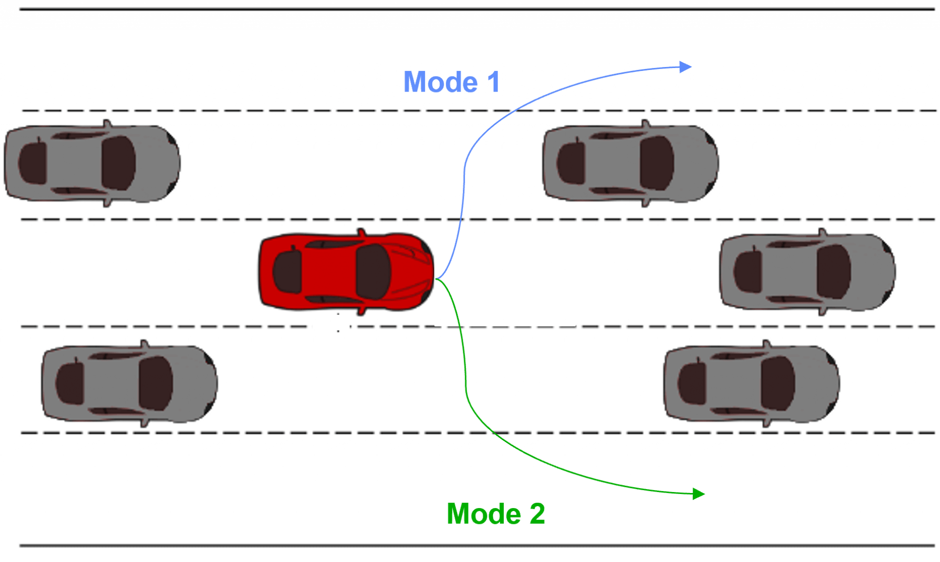
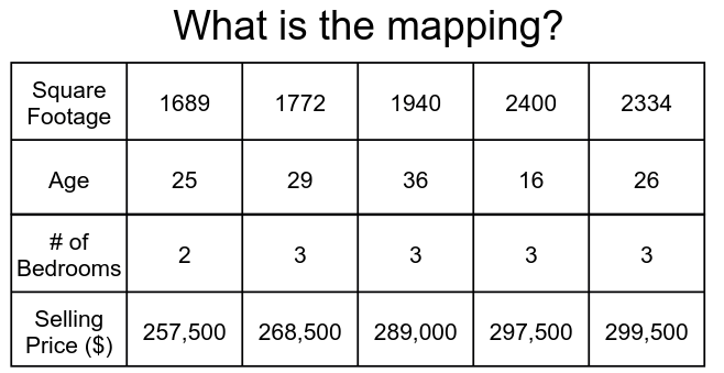
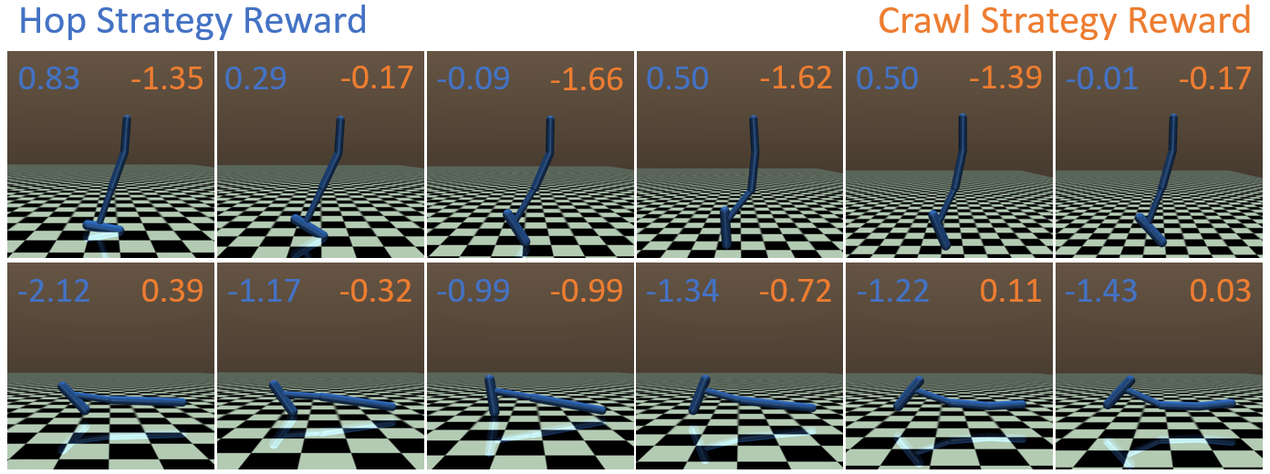
Gradient descent is an ubiquitous optimization algorithm used to train machine learning (ML) algorithms from simple linear regression models to sophisticated transformer architectures. ML researchers are typically introduced to unconstrained optimization problems (e.g., least-squares, LASSO, or Ridge regression). However, many really-world ML problems are constrained optimization problems. For example, in robotics, we may want to train a robot for maneuvering around a crowd by imitating human motion (e.g., Behavior Cloning where the robot minimizes the divergence between the distribution of actions the robot takes and that the human would take in the same state of the world, $x$) subject to the constraint that the robot will never crash into a person.

In this blog post, we will look at some powerful approaches for performing constrained optimization. First, we quickly recap the concept of gradient descent. Next, we’ll delve into Projected Gradient Descent, a technique that introduces constraints to the optimization process. Finally, we’ll uncover the magical world of Mirror Gradient Descent, a method that combines the power of duality and optimization. For an example of how Mirror Gradient Descent has been used, check out these papers:

• Montgomery, W.H. and Levine, S., 2016. Guided policy search via approximate mirror descent. Advances in Neural Information Processing Systems, 29.
• Zhang, M., Geng, X., Bruce, J., Caluwaerts, K., Vespignani, M., SunSpiral, V., Abbeel, P. and Levine, S., 2017, May. Deep reinforcement learning for tensegrity robot locomotion. In 2017 IEEE international conference on robotics and automation (ICRA) (pp. 634-641). IEEE.
• Cheng, C.A., Yan, X., Wagener, N. and Boots, B., 2018. Fast policy learning through imitation and reinforcement. arXiv preprint arXiv:1805.10413.

Recap: Gradient descent
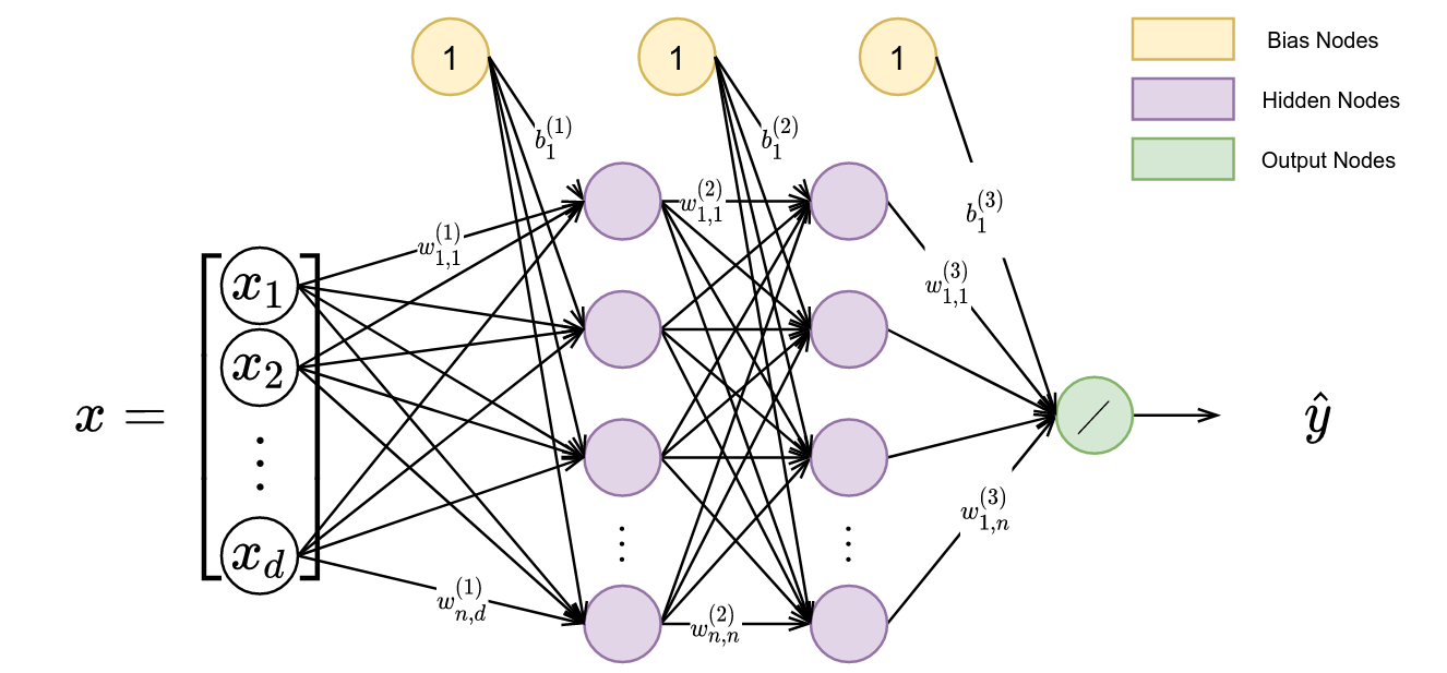
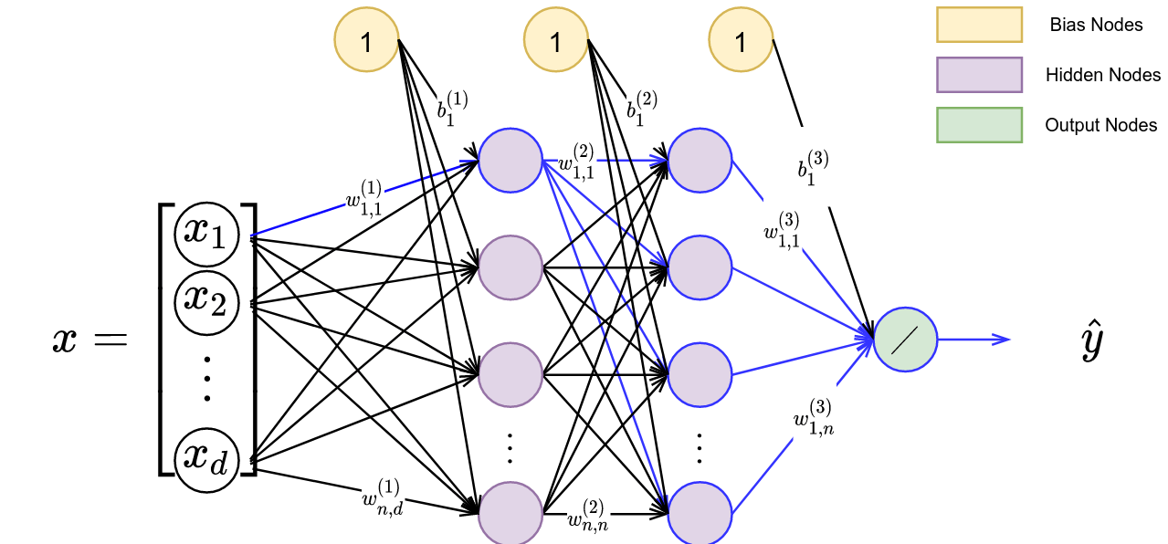
Imagine we are trying to train a neural network with a parameter \(\theta\). Given \(\theta\), the neural network produces the prediction \(f(\theta)\). We have a cost function \(\mathcal{L}(\theta)\). Our goal is to find the optimal parameter $\theta^*$ that minimizes \(\mathcal{L}(\theta)\). Let’s consider the standard \(L^2\)-norm loss function with respect to our dataset \(D\), defined as follows:
\[\mathcal{L}(\theta) = \Sigma_{(x,y) \in D} \frac{1}{2} ||y-f_\theta (x)||^2 .\]

Starting from an initial point \(\theta_0\), Gradient Descent performs the following update at every timestep:
\[\theta_{t+1} \leftarrow \theta_t -\alpha \nabla_\theta \mathcal{L}(\theta_t).\]

Note that we are going opposite to the gradient direction (minus sign in the gradient) since we are “minimizing” the loss function. When the dataset is too large to compute the gradient at every timestep, we use Stochastic Gradient Descent which computes the gradient with respect to a single example, or Mini-batch Gradient Descent which computes the gradient with respect to a small batch sampled from the dataset at every timestep.

For more information such as time complexity and convergence rate, please refer to our previous blog post: Bootcamp Summer 2020 Week 1 – Gradient Descent.

Constrained Optimization Problem
In many real-world scenarios, optimization problems are often attached to certain constraints or boundaries that resulting parameters must satisfy. These constraints can represent physical limitations, practical considerations, or desired properties of the solutions. For example, consider a manufacturing company that produces various products. The company aims to maximize the overall utility derived from these products, taking into account factors such as customer demand, quality, and profitability. However, the company faces a budget constraint, which limits the total amount of money available for production.

To formulate this as a constrained optimization problem, let’s first define the following variables:
$x_1, \cdots, x_n$: The quantities of each product to be manufactured.
$U(x_1, \cdots, x_n)$: The utility function that quantifies the overall satisfaction derived from the products.
$c_1, \cdots, c_n$: The respective costs of producing each product.

The objective is to maximize $U(x_1, x_2, \cdots, x_n)$ while satisfying the constraint of the total budget, $B$. Mathematically, the constrained optimization problem can be formulated as:

\begin{align*}
Maximize_{x_1, \cdots, x_n} \text{ } & U(x_1, \cdots, x_n)\notag\\
\text{subject to } & \Sigma_{i=1}^n x_i*c_i \leq B.\notag
\end{align*}

This example highlights the need for algorithms to solve such constrained optimization problems that arise in various fields, such as resource allocation, portfolio optimization, and image reconstruction.

Projected Gradient Descent

Then, how can we incorporate the constraints into the optimization process so that we can balance between optimizing the objective function and constraining parameters? Projected Gradient Descent (PGD) addresses this challenge by ensuring that the iteratively updated parameters belong to the feasible region defined by the constraints.

The key idea behind PGD is to project the current solution onto the feasible region at each iteration. This projection step involves mapping the updated parameter onto the closest point within the feasible region in case if lands outside of it, effectively “projecting” it onto the constraint boundaries. By doing so, PGD guarantees that the resulting parameters remain feasible throughout the optimization process.

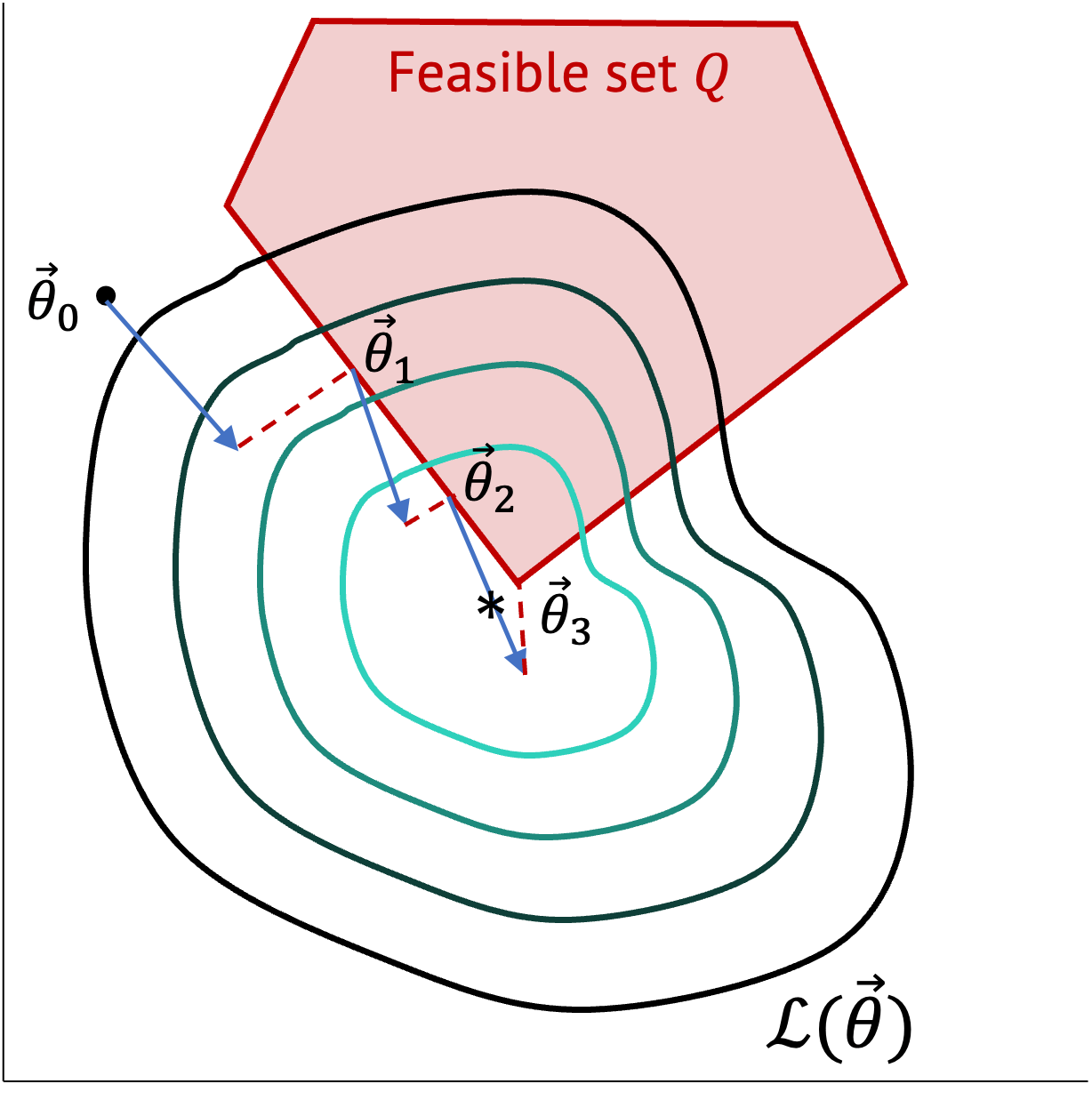
To illustrate, let’s consider a constraint \(A\theta = b\) for our optimization problem. Assume Q is the feasible set for the constraint (the red region from Fig. 1) and P is the projection function onto $Q$:

\[Q = \{\theta|A\theta = b\},\]
\[P: \theta’ \mapsto arg\,min_{\theta \in Q} \frac{1}{2} ||\theta – \theta’||^2 .\]

Projected gradient descent is defined as follows:

\[\theta_{t+1} \leftarrow P(\theta_t – \alpha_t \nabla_\theta \mathcal{L}(\theta_t)).\]

For the Lipshitz constant \(L\) and the step-size \(\alpha_t = \frac{R/G}{\sqrt{t}}\), it is known that if \(R \geq ||\theta_0 – \theta||_2\) and the gradient of \(\mathcal{L}\) is bounded by a constraint \(G\), i.e., \(G \geq ||g||_2\), \(\forall g \in \frac{\partial \mathcal{L}}{\partial \theta}\), the inequality \(\mathcal{L}(\theta_t) – \mathcal{L}(\theta^*) \leq C \frac{L}{\sqrt{t}}\) holds.

Mirror Gradient Descent

Mirror Gradient Descent (MGD) is a fascinating optimization technique that combines the power of optimization with the concept of duality. It draws inspiration from convex duality, a fundamental concept in convex optimization that establishes a relationship between primal and dual problems. MGD exploits this duality to transform the original optimization problem into a dual problem and solves it using a gradient descent-like approach.

In MGD, the optimization process involves iteratively updating the primal parameter in the primal space, while simultaneously updating the corresponding dual parameter in the dual space. The updates are performed by taking steps in the direction opposite to the gradients of the primal and dual objectives. This dual update is analogous to a mirror reflection of the primal update, which is the reason why this algorithm is called by the name “Mirror Gradient Descent.”

The motivation to work in the dual space is that it can often be simpler or have desirable geometric or algebraic properties, leading to more efficient optimization. MGD has been applied to various domains, including convex optimization, machine learning, and signal processing. It offers a powerful framework to tackle optimization problems with complex constraints or objectives, leveraging the interplay between primal and dual updates to achieve efficient convergence and desirable parameters.

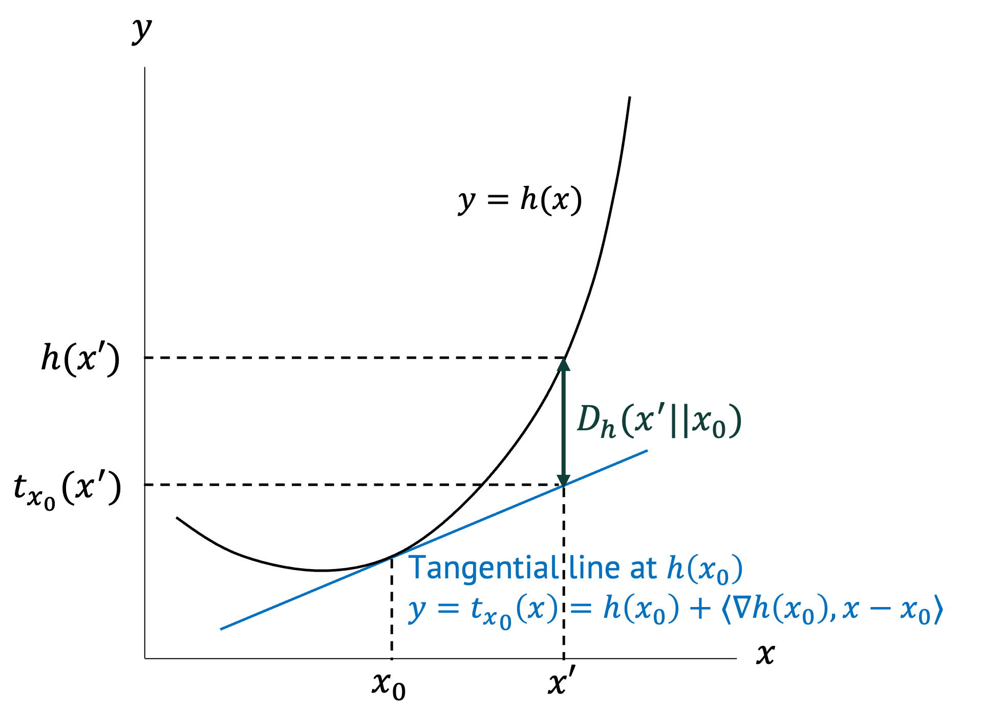
Before we dig into MGD more, let’s first define Bregman Divergence of a function \(h\) as \(D_h (x’||x)\).

\[D_h (x’||x):= h(x’)-h(x)-\langle \nabla h(x), x’-x \rangle \]
(\(\langle \cdot,\cdot \rangle\) is dot product.)

If we do the first order Taylor expansion of a function $h$, the tangential line at \(h(x)\) crosses a point \((x’, h(x) + \langle \nabla h(x), x’-x) \rangle) \). Bregman Divergence \(D_h (x’||x)\) is the gap between \(h(x’)\) and \(h(x) + \langle \nabla h(x), x’-x) \rangle \). It becomes large when the function \(h\) is steeper.

Mirror gradient descent is defined as follows:
\[\theta_{k+1} \leftarrow arg\,min_\theta {\langle \alpha_k \mathcal{L}(\theta_k), (\theta – \theta_k) \rangle + D_h (\theta||\theta_k)}. \]

The concept of mirror gradient descent is that we first transform (with \(\nabla h(\theta_k)\)) the primal space of \(\theta\) into the dual space of \(\phi\) which possibly have an easier geometry, update the parameter, and do inverse-transform to come back to the primal space.

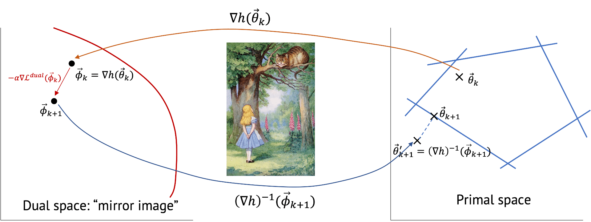
Now, let’s first get a mirror image in the dual space and then project it back (with \((\nabla h)^{-1} (\phi_{k+1}))\) to the primal space.

\begin{align*}
0 & = \frac{\partial}{\partial \theta} \{\alpha \langle \nabla \mathcal{L}(\theta_k), \theta_{k+1}-\theta_k \rangle + h(\theta_{k+1}) – h(\theta_k) – \langle \nabla h(\theta_k), \theta_{k+1} – \theta_k \rangle \} \\
& = \alpha \nabla \mathcal{L}(\theta_k) + \nabla h(\theta_{k+1}) – \nabla h(\theta_k)
\end{align*}

Finally, we get the update equation for mirror gradient descent:
\[\nabla h(\theta_{k+1}) = \nabla h(\theta_k) – \alpha \nabla \mathcal{L}(\theta_k) \]
\[ \theta_{k+1} \leftarrow (\nabla h)^{-1} [\nabla h(\theta_k) – \alpha \nabla \mathcal{L}(\theta_k)]. \]

Note that for constrained optimization program, the projection onto the feasible set can be applied afterward.

Example 1. For \(h(\theta)=\frac{1}{2}||\theta||^2\), Bregman Divergence becomes \(D_h(\theta||\theta_k) = \frac{1}{2} ||\theta-\theta_k||^2 \). Substituting Bregman Divergence and rewriting the update equation, we get

\[\theta_{k+1} \leftarrow arg\,min_\theta \{ \langle \alpha_k \nabla_\theta \mathcal{L}(\theta_k), (\theta – \theta_k)\rangle + \frac{1}{2} ||\theta – \theta_k||^2 \}.\]
Then,

\begin{align*}
0 & = \nabla_\theta f = \frac{\partial f}{ \partial \theta} \\
& = \frac{\partial}{\partial \theta} \{\langle \alpha_k \nabla_\theta \mathcal{L}(\theta_k), (\theta – \theta_k) \rangle + \frac{1}{2} ||\theta – \theta_k||^2\} \\
& = \frac{\partial}{\partial \theta} \langle \alpha_k \nabla_\theta \mathcal{L}(\theta_k), \theta \rangle – \frac{\partial}{\partial \theta} \langle \alpha_k \nabla_\theta \mathcal{L}(\theta_k), \theta_k \rangle + (\theta-\theta_k) \\
& = \alpha_k \nabla_\theta \mathcal{L}(\theta_k) + (\theta-\theta_k)
\end{align*}

which corresponds to the basic gradient descent \(\theta_{k+1} = \theta_k – \alpha_k \nabla_\theta \mathcal{L}(\theta_k) \). Indeed, gradient descent is a special case of mirror gradient descent with this \(h\). Another intuition for recognizing it is that for \(h(\theta)=\frac{1}{2}||\theta||^2\), \(\nabla_\theta h = \theta, (\nabla_\theta h)^{-1} = \theta \), i.e., the transform is one-to-one mapping. Hence, we get \(\theta_{k+1} = \theta_k – \alpha \nabla \mathcal{L}(\theta_k) \).

Example 2. \(h(\theta) = \Sigma_i \{\theta_i \ln(\theta_i) – \theta_i\} \) where $\theta$ satisfies \(\Sigma_i \theta_i = 1\).

\[\nabla h = [\ln(\theta_1), …, \ln(\theta_n)]^T, (\nabla h)^{-1} = \exp (\theta) \]

\[\langle \nabla h(\theta), \theta’ – \theta \rangle = \Sigma_i \frac{\partial h}{\partial \theta_i} (\theta’_i – \theta_i) = \Sigma_i (\ln \theta_i) (\theta’_i – \theta_i)\]

\[\Rightarrow D_h (\theta’||\theta) = \Sigma_i \{\theta’_i \ln(\frac{\theta’_i}{\theta_i}) – \theta’_i +\theta_i\} = \Sigma_i \theta’_i \ln(\frac{\theta’_i}{\theta_i})\]
using $\Sigma_i \theta_i = \Sigma_i \theta’_i = 1$. Note that with this $h$, Bregman Divergence converges to KL Divergence.
The update equation for mirror gradient descent becomes
\[\theta^{i}_{k+1} \leftarrow \exp(\ln(\theta_k) – \alpha \nabla \mathcal{L}(\theta_k)) = \theta_k \exp(-\alpha \nabla \mathcal{L}(\theta_k))\]

Typically, it’s good to use mirror descent if you are able to pick a good \(h\) for that class of problems.

There are also many other variants of gradient descent. Each algorithm possesses unique strengths, you may try to find what suits the best for your own optimization problem. Understanding and utilizing these techniques expands our problem-solving capabilities across diverse fields. So, please feel free to embrace these algorithms and explore their potential in your own endeavors.

Conclusion

Projected and Mirror Gradient Descent are powerful tools for constrained optimization problems in ML. These algorithms are more computationally expensive that regular gradient descent due to their need to address the constraints. The Bregman Divergence is an expressive way to represent many forms of optimization (e.g., Examples 1 and 2). Constrained optimization is key in safety-critical domains, such as ML for robotics and healthcare where constraint satisfaction must be enforced. Note: check out our blog post on KKT conditions for an alternative approach for constrained optimization: The method of Lagrange Multipliers.

Acknowledgements

This blog post was developed in part with support from course materials available at http://www.cs.cmu.edu/afs/cs.cmu.edu/academic/class/15850-f20/www/notes/lec19.pdf

Imagine we have an autonomous car that would like to perform speedy highway driving. There are several approaches to program such an autonomous vehicle. The first would be to hand-craft a rule-based system consisting of what to do in different scenarios. An example rule could be “if the autonomous car would like to move forward and there is a car in front and to the left, switch to the right lane”. A programmer could write down hundreds of rules consisting of every possible scenario. However, this process is expensive and leaves much to be desired. The second approach would be to utilize a driving simulator and design a reward function that defines the proper autonomous driving behavior. Then, one could use reinforcement learning to learn an optimal driving policy. However, defining such a reward function is difficult. Furthermore, if the driving simulator has differences with the real world, the behavior of the autonomous car may degrade when deployed. Lastly, one can utilize learning from demonstration (LfD), where user demonstrations are used directly to learn autonomous driving behavior. LfD has many benefits, including that it can learn human-like behavior and does not require a simulator. It is also much easier for a human to give an example of driving on the highway than defining all the rules used during driving. However, what happens when two drivers present demonstrations with conflicting behaviors (e.g., one prefers to pass on the left versus the other prefers to pass on the right)?

In this post, we are going to discuss how robots can learn from heterogeneous human demonstrators, demonstrators that will perform the same task in different ways.

This blog post will address the following questions in 3 parts:

1. What challenges arise from heterogeneity in demonstrations?
2. How can we automatically infer preferences within demonstrations?
3. How can we utilize person-specific embeddings in policy learning?

1. Challenges from heterogeneity of demonstrations

We can imagine multiple real-life scenarios, ranging from driving to the setting of a dinner table, in which there are heterogeneous approaches that can be utilized to reach the same goal. Continuing the autonomous driving example from the introduction, Figure 1 displays the heterogeneity that can occur within driving demonstrations. Within the example displayed, some subset of the demonstrators preferred to pass on the left while others preferred to pass on the right. LfD approaches that assume homogeneous demonstration will either fit to the mean (drive straight into the car in front) or fit a single-mode (only pass on one side), both producing suboptimal/limited driving behavior. It is important to model the heterogeneity within the Learning from Demonstration framework. We will accomplish this via variational inference for person-specific embeddings.

The decision-making we employ to select our approach can be explicitly defined as a policy; a function that maps states $S$ to actions $A$ (Equation 1).

\begin{align}
\hat{\pi}: S \rightarrow A
\end{align}

Depending on an implicit demonstrator preference, the demonstrator may find it advantageous to choose one policy over the other. For example, a demonstrator setting the table may be left-handed and prefer to set a drinking glass on the left-hand side. Without explicitly labeling demonstrations by preference, the context within this selection process is lost to a robot attempting to learn the task, making it very difficult to learn a policy representation across all demonstrators. Without access to latent information about demonstrators, current LfD approaches sacrifice optimal behavior for consistency, weaken the robustness of the robot to different scenarios, and reduce the number of examples the robot can use to learn from.

As we consider scenarios where the number of demonstrations is numerous, it becomes advantageous to be able to autonomously infer distinct modalities without requiring someone at hand to label each demonstration. In addition, we would also like to learn a policy representing user demonstrations within our dataset. How can one accomplish both objectives, inferring latent information about demonstrated trajectories and learning a policy conditioned upon contextual and latent information, simultaneously?

2. Inferring trajectory modalities

We seek to autonomously infer distinct strategies or modes $\omega$ from the real-world demonstrations we are able to acquire. Following our autonomous driving example, Figure 2 displays the end result we seek to achieve: mode 1 demonstrations are assigned a specific latent code and mode 2 demonstrations are assigned a different latent code. Visually, in Figure 2 it is clear that there are only two types of demonstrations. We would like our approach to discover first, that there are different modes within the demonstration data-set and second, how many modes are present.

To do so, we would like to maximize the mutual information $I$ between our embedding mode $\omega$ and the actions taken by our policy $\pi_\theta(a|\omega,s)$, where our policy is conditioned on the state and latent code. We display a representation of the mutual information in Equation 2, where H is the entropy function.

\begin{gather}
I(\omega;\pi(a|\omega,s)) = H(\omega) – H(\omega|\pi(a|\omega,s))
\end{gather}

Maximizing mutual information encourages $\omega$ to correlate with semantic features within the data distribution (i.e., mode discovery), which is exactly what we want! However, maximizing the mutual information between the trajectories and latent code is intractable as it requires access to the true posterior, $P(\omega|s,a)$, representing the distribution of modalities given trajectories. Instead, we can utilize a lower bound of the mutual information and maximize the lower-bound via gradient descent, thereby maximizing the mutual information and incentivizing the policy to utilize $\omega$ as much as possible.

Recall that the KL divergence is a measure of similarity between two probability distributions. We can express the KL divergence between $p$ and $q$ with Equation 3.

\begin{align}
D_{KL} \left( p (\omega | s, a) \ || \ q(\omega | s, a) \right) = \mathop{\mathbb{E}}_{\omega \sim p(\omega | s, a)} log \frac{p(\omega | s, a)}{ q(\omega|s,a)}
\end{align}

We display the derivation of the mutual information lower bound in Equation 4. Below, we provide a step-by-step walkthrough of the derivation.
\begin{align}
\begin{split}
I(\omega;\pi(a|\omega,s)) &= H(\omega) – H(\omega|\pi(a|\omega,s))) \\
&= H(\omega)-\mathop{\mathbb{E}}_{a \sim \pi(\cdot| \omega, s)}\big[\mathop{\mathbb{E}}_{\omega \sim p(\omega| s,a)} [- \log p(\omega|s,a)\big]] \\
&= H(\omega)+\mathop{\mathbb{E}}_{a \sim \pi(\cdot| \omega, s)}\big[\mathop{\mathbb{E}}_{\omega \sim p(\omega| s,a)} [\log p(\omega|s,a)\big]] \\
&= H(\omega)+D_{KL}(p(\omega|s,a)||q(\omega|s,a)) + \mathop{\mathbb{E}}_{a \sim \pi(\cdot| \omega, s)}\big[\mathop{\mathbb{E}}_{\omega \sim p(\omega| s,a)} [\log q(\omega|s,a)\big]] \\
&\geq H(\omega) + \mathop{\mathbb{E}}_{a \sim \pi(\cdot| \omega, s)}\big[\mathop{\mathbb{E}}_{\omega \sim p(\omega| s,a)} [\log q(\omega|s,a)\big]] \\
\end{split}
\end{align}

In line 1 of the derivation, we have Equation 2. To transition into line 2 of the derivation in Equation 4, we simplify the second entropy term. Line 3 of the derivation brings the negative sign outside of the expectation. Line 4 utilizes the identity $\mathop{\mathbb{E}}_{x \sim p_{X}(\cdot)}(p(x)) = D_{KL}(P||Q) + \mathop{\mathbb{E}}_{x \sim p_{X}(\cdot)}(q(x))$ in transitioning from line 3. Here, q is an approximate posterior for the true distribution of embeddings given trajectories. In transitioning to line 5, since the KL divergence between two distributions is always positive, we replace the equal sign with a greater than or equal to and remove the divergence term. We note that during optimization, we assume that the distribution of embeddings is a static, uniform distribution, and thus, the entropy across latent codes, $H(\omega)$ is constant and can be removed. Line 5 displays the final result, the lower bound of the mutual information.

Notice that we have now described a substitute objective function that is expressly in terms the latent mode variable $\omega$ and our approximate posterior $q$. Maximizing this objective should make different latent embeddings correspond with different policy behaviors. However, one problem remains: our computation of $q$ is based on the sampling over the expectation of the true posterior p($\omega$|s,a), which is still unknown. Therefore, we seek to gradually tease out the true distribution while training through sampling. We denote $\omega$, the discovered latent codes, as person-specific embeddings as each embedding displays latent features for a specific demonstrator.

3. Simultaneously learning a policy while inferring person-specific embeddings

Our goal is to learn demonstrator policies that are conditioned on person-specific embeddings, $\omega$. Thus, even if heterogeneity is present with the demonstrations, the latent encodings will be able to represent the unique behaviors among demonstrators. The resultant policy is able to adapt to a person’s unique characteristics while simultaneously leveraging any homogeneity that exists within the data (e.g., uniform adherence to hard constraints).

Accordingly, we will want to maximize our ability to imitate demonstrators via a behavior cloning loss and the mutual information between person-specific embeddings and trajectories via a variational information maximization (VIM) loss. We display a general overview of the architecture used during learning from heterogeneous demonstration in Figure 3.

In this figure, we have a policy represented by $\pi$ and parameterized by $\theta$, and an approximate posterior represented by $q$ and parameterized by $\phi$. We start with a set of person-specific embeddings initialized uniformly. As training proceeds, we infer the person-specific embeddings ($\omega$ is a learned latent encoding via gradient descent) and learn a policy representing all demonstrators. We display a sample algorithm in Figure 4 for learning $\theta$, $\phi$, and $\omega$.

In step 1 of the algorithm, we sample from the set of demonstrators and obtain the trajectories associated with the sampled demonstrator. We initialize a new embedding, $\omega^{(i)}$, for the demonstrator. In step 2 and 3, we conduct a forward pass through the architecture displayed in Figure 3 and update parameters $\theta$ and $\omega$ via both the behavior cloning and VIM loss. In step 4, we utilize the VIM cost function to update $\phi$. We repeat this process until convergence. Once the algorithm has converged, every demonstrator’s person-specific embedding will accurately represent their modality. Utilizing this latent embedding within the learned policy will produce a representation of the demonstrator’s behavior.

In conclusion, the main takeaways from our blog post are as follows:

1. It is important to model the heterogeneity when Learning from Heterogeneous Demonstration (LfHD). We present a framework that can adapt to a person’s unique characteristics while simultaneously leveraging any homogeneity within the data.
2. We infer person-specific latent embeddings with semantic meaning by maximizing the lower bound of the mutual information between an inferred latent variable and a policy that is conditioned upon the latent variable.

Further Details

If you want to explore more on this, feel free to check our recent NeurIPS paper.

Previously, we covered gradient descent, an optimization method that adjusts the values of a set of parameters (e.g., the parameters of a linear regression model) to minimize a loss function (e.g., the mean squared error of a linear regression model network in predicting the value of a home given its zip code and other information). In this post, we introduce neural networks, which are essentially hyperparameter function approximators that learns to map a set of inputs to a set of outputs.

To optimize a neural network model with respect to a given loss function, we could directly apply gradient descent to adapt the parameters of a neural network to learn a desired mapping of inputs to outputs, this process would be inefficient. Due to the large number of parameters, performing symbolic differentiation as introduced in our gradient descent lesson would require a lot of redundant computation and slow down the optimization process tremendously. Fortunately, there is a better way: the backpropagation algorithm. Backpropagation is a form of auto-differentiation that allows us to more efficiently compute the derivatives of the neural network (or other model’s) outputs with respect to each of its parameters. Backpropagation is often overlooked or misunderstood as a simple application of symbolic differentiation (i.e., the chain rule from Calculus), but it is much, much more.

This blog will cover

1. Neural Networks
2. Forward Propagation
3. Backpropagation

We will not take the time to discuss the biological plausibility of neural networks, but feel free to check out this paper.

Neural Networks

We will start by understanding what a neural network is. At its core, a neural network is a function approximator. Functions from algebra, such as $y=x^2$ and $y=2x+1$, can be represented by neural networks. Neural networks can be used to learn a mapping given a set of data. For example, a neural network could be used to model the relationship of the age of a house, the number of bedrooms, and the square footage with the value of a house (displayed in Figure 1).

While the example in Figure 1 may appear trivial, neural networks can solve much more challenging problems. For example, neural networks have been applied to take as input Magnetic Resonance Imaging (MRI) data and output diagnoses for the patient based upon what is present in the MRI. Neural networks have also had success in being applied to problems of “machine translation” in which one attempts to translate one language to another (e.g., English to Chinese).

Typically, neural networks are given a dataset $\mathcal{D}=\{(x_k,y_k),\ k\in [n]\}$, where $(x_k,y_k)$ is the   “example” number $k$, $x_k$ is the input to a model we want to train, and $y_k$ is the “label” we want our model to learn to predict from $x_k$. We generalize the notation to $x$ being the input data, and $y$ being the set of ground-truth labels. A neural network can be represented as a function $\hat{y} = f(x)$ (i.e., $f: X \rightarrow Y$). Here, we use “$\hat{y}$” as the output of the neural network instead of “$y$,” as $\hat{y}$ is our estimate of the ground-truth label, $y$. Later, we will use the difference (i.e., error) between $\hat{y}$ and $y$, to optimize our neural network’s parameters.

If we look inside the function $f$, we see nodes and edges. These nodes and edges make up a directed graph, in which an input is operated on from left to right.

A closer look inside a smaller neural network is shown in Figure 2. Figure 2 displays how an input, $x$ (with cardinality $|x|=d$), is mapped to an output, $\hat{y}$, a scalar. Before we move into what is happening here, let’s will first explain the notation.

We have neural network weights, denoted by $w$, that weight the incoming value through multiplication. The subscripts represent the (to, from) nodes respectively, and the superscript denotes the layer number resulting in the notation as $w^{(layer)}_{to,from}$. The terms with the number “1” inside are termed bias nodes and are represented in the notation “b_{to}”.

As an example, we present a simple neural network describing $\hat{y} = 2x + 4z +3$ in Figure 4.

When an input is passed into a neural network, the input $x$ is multiplied by respective weights (denoted by $w$) and added to by a bias term $b$, resulting in a new value represented within a hidden node. In our model, we set the number of nodes in each layer to $n$. Each node, along with its incoming edges, represents some inner function. As our neural network can have many nodes and many layers, neural networks can be thought of as a composition of these inner functions to produce a more complex, outer function $f$ described above. The backslash in the most-right node represents a summation, resulting in a scalar value output. Now we will discuss precisely how to produce an output $\hat{y}$ given an input $x$ through learning a mapping.

Forward Propagation

The final output $\hat{y}$ is computed from the node values and weights of the previous layer, in our case, layer 2. We can multiply the output of the hidden nodes in layer 2, denoted by $o^{(2)}_i$, where $i$ represents a node index from $i$ to $n$ (i.e., $i \in \{1,2,\ldots,n\}$, by the weights connecting these nodes with the output node and add the bias term b^{(3)}_{i}. We display this process in Equation 1.

\begin{align}
\hat{y} = \sum_{i=1}^n w_{1,i}^{(3)} o^{(2)}_i + b^{(3)}_{1}
\end{align}

But, what is $o_i^{(2)}$ equal to? We display how $o_i^{(2)}$ is computed in Equation 2.

\begin{align}
o_i^{(2)} = g(z_i^{(2)})
\end{align}

Here, $i$ is again the node index and $g$ is an activation function (i.e., $g: Z \rightarrow O$). Neural networks cannot represent nonlinear functions without utilizing nonlinear activation functions. Activation functions help neural networks represent more complex functions by transforming node values by a nonlinear function. Common activation functions used include ReLU, tanh, sigmoid, etc. Here, we will discuss and use the ReLU (Rectified Linear Unit) as our activation function.

For our example, we will use the ReLU activation function, as shown in Equation 3.

\begin{equation}g(z) =\bigg\{\begin{aligned} &z \text{ if }z \geq 0\\ &0 \text{ otherwise}\end{aligned}\bigg\}\end{equation}

It is also helpful to know the gradient of the ReLU function, displayed in Equation 4.

\begin{equation}g'(z) =\bigg\{\begin{aligned} &1 \text{ if }z \geq 0\\ &0 \text{ otherwise}\end{aligned}\bigg\}\end{equation}

Moving back to Equation 2, we solve for $z_i^{(2)}$ in Equation 5.

\begin{align}
z^{(2)}_i = \sum_{j=1}^n w_{i,j}^{(2)} o^{(1)}_j + b^{(2)}_{i}
\end{align}

This procedure can be used throughout the neural network, computing the current layer using the previous layer’s output. For simplicity of algorithmic notation, you can consider the neural network’s input, $x$, as $o^{(0)}$. Here, $o^{(0)}$ represents the hypothetical output of a hypothetical zeroth layer. In Algorithm 1, we display the complete forward propagation algorithm, expressing the layer number as a variable for generalizability. This algorithm computes a predicted output, represented by $\hat{y}$, given input features, $x$.

We can now analyze the computational complexity of this algorithm. For the sake of simplifying the analysis, we assume the number of layers in the neural network, $l$, is equal to the number of nodes in each layer, $n$, which we also set as equal to the size of the input, $|x|=d$. Thus, $n=l=w$. In Algorithm 1, Steps 3 and 5 represent a matrix multiplication combined with addition. This process has a complexity of $O(n^2+n)$. As a reminder, for any matrix multiplication of two matrices of size $p \times q$ and $q \times r$, respectively, the computational complexity of this multiplication is $O(pqr)$. Thus, since we are multiplying weight matrices of size $n \times n$ to a vector of size $n \times 1$, the complexity of the matrix multiplication alone is $O(n \times n \times 1) = O(n^2)$. The addition operation adds complexity $O(n)$, resulting in $O(n^2+n)$ for Steps 2-6. Steps 8-10 have a complexity of $O(n)$ leading, resulting now in the complexity $O(n^2 + 2n)$. Since Step 1 iterates $n=l$ times, we arrive at a total complexity of $O(n(n^2 + 2n))=O(n^3)$ for Algorithm 1.

Now that we can perform a forward pass and know its complexity, we can discuss how to update our weights and attempt to learn a model that fits the data.

Backpropagation

To optimize our neural network weights to more accurately represent our data, we first establish a loss function that quantifies our model’s error (i.e., how wrong its outputs are for a desired task). Given this loss function, we could then compute the gradients of our loss function with respect to each weight. We could then perform gradient descent to optimize our model parameters as we did in the gradient descent blog post. However, we will now do something a bit more sophisticated to make the optimization process more computationally efficient.

Let’s consider a common loss function, as shown in Equation 6. This loss function represents a mean-squared error loss between the true label (true y-value in the data) and the predicted value using our neural network ($\hat{y}$).

\begin{align}
L=\frac{1}{2} (y-\hat{y})^2 = \frac{1}{2} (y-f(x))^2
\end{align}

The derivative of this loss function with respect to $w_{1,1}^{(1)}$ is displayed in Equation 7 according to chain rule.

\begin{align}
\frac{\partial L}{\partial w_{1,1}^{(1)}} = (y-\hat{y}) * \frac{\partial \hat{y}}{\partial w_{1,1}^{(1)}} \bigg|_x
\end{align}

So, how do we comput $\frac{\partial \hat{y}}{\partial w_{1,1}^{(1)}}$? There are 4 paths from the output node to $w_{1,1}^{(1)}$, which highlighted in blue in Figure 4. The upper-most path has the gradient shown in Equation 8.

\begin{align}
\frac{\partial \hat{y}}{\partial w_{1,1}^{(1)}} =  \frac{\partial \hat{y}}{\partial o^{(3)}} \frac{\partial o^{(3)}}{\partial z^{(3)}} \frac{\partial z^{(3)}}{\partial o^{(2)}_1} \frac{\partial o^{(2)}_1}{\partial z^{(2)}_1} \frac{\partial z^{(2)}_1}{\partial o^{(1)}_1} \frac{\partial o^{(1)}_1}{\partial w_{1,1}^{(1)}}
\end{align}

The rule for computing the “total derivative” encompassing all of these paths can be seen through an example here.

Computing a single partial derivative is computationally expensive, and computing each weight’s partial derivative individually (e.g., (e.g., $\frac{\partial \hat{y}}{\partial w_{1,1}^{(1)}}$ and then $\frac{\partial \hat{y}}{\partial w_{1,2}^{(1)}}$) and so forth all the way to $\frac{\partial \hat{y}}{\partial w_{1,n}^{(l)}}$) would be terribly inneficient.

If we instead look at $\frac{\partial \hat{y}}{\partial w_{1,2}^{(1)}}$, you can see that it shares many of the same nodes as $\frac{\partial \hat{y}}{\partial w_{1,1}^{(1)}}$. In Figure 5, we display a depiction of gradient computations required for $w_{1,1}^{(1)}$, $w_{2,1}^{(1)}$, and the overlap in the computations.

We would like to take advantage of this overlap in computation, which is exactly where the Backpropagation algorithm comes in. Backpropagation is a form of reverse-mode automatic differentiation that allows us to eliminate redundant computation in applying the chain rule to compute the gradient of our neural network.

Applied to neural networks, the backpropagation algorithm starts from the last layer of the neural network, computes an error term (denoted as $\delta$), and multiplies this error term by the gradient. The algorithm computes each node’s respective gradient in memory and reuses these variables as the algorithm continues, backpropagating the information for efficiency. We display the algorithm for Backpropagation in Algorithm 2. The output of the Backpropagation algorithm is gradients for each set of weights and biases.

Looking at the computational complexity of this algorithm, we see Step 4 has a complexity of $O(1)$. Step 6 has a complexity of $O(n^2 + n)$ or $O(n^2)$. Step 10 has a complexity of $O(n)$. Steps 12 and 14 both have complexities of $O(n^2)$. Since we iterate over the number of layers, equal to $n$ for our analysis, the total complexity is $O(n^3)$. If we did not use the Backpropagation algorithm, we would end up redundantly computing each component’s derivatives multiple times. Using the previous assumptions setting the cardinality of $|x|$, the number of nodes, and the number of layers to $n$, we would be iterating over $O(n^3 + n^2)$ weight derivatives resulting in a total complexity of $O(n^6)$.

The last step in optimizing our neural network model to minimize our loss function is to update weights and biases. Equations 9-10 show one step of gradient descent using the derivatives from our backpropagation procedure in Algorithm 2. Note that Equations 9-10 represent only one step of gradient descent, so one would need to iteratively perform the forward pass, then backward pass, then parameter updates (Equations 9-10) until the model converges to a local minimum, as described in our previous post on gradient descent.

\begin{align}
w^{(l)} \to w^{(l)} + \alpha \Delta w^{(l)}
\end{align}
\begin{align}
b^{(l)} \to b^{(l)} + \alpha \Delta b^{(l)}
\end{align}

We now have the ability to train neural networks in a computationally efficient manner, which, in turn, allows us to do more training iterations per unit time, which should help us train more accurate neural networks!

Key Points throughout this Blog:

1. Neural networks can be used to represent almost any function.
2. Forward propagation is the process of taking input features, $x$, and computing an output in the form of a model’s estimate, $\hat{y}$.
3. We can use the difference in the output, $\hat{y}$, of the neural network and our ground-truth data, $y$, to compute a loss, and then use this loss value to compute gradients in the backpropagation algorithm.
4. Backpropagation is a special case of reverse-mode automatic differentiation and allows for efficient gradient computation. The result is that the training of extremely large neural networks is possible!